6. Landslide prediction using time series of displacement
Pascal LACROIX1 & Diego CUSICANQUI1
1 Univ. Grenoble Alpes, CNES, CNRS, IRD, Institut des Sciences de la Terre (ISTerre), Grenoble, France.
Copyright
Document version 0.2, Last update: 2025-09-18
© PSF TelRIskNat 2025 Optical team (D. Cusicanqui, R. Basantes & P. Lacroix). This document and its contents are licensed under the Creative Commons Attribution 4.0 International License (CC BY-NC-SA 4.0).
6.1. Learning objectives:
Visualize time-series of landslide displacements from different sensors.
Predict the occurrence time of a landslide failure.
Understand the notions of uncertainties on landslide displacements.
6.2. Introduction
Landslides are a major threat in most mountainous environments of the world provoking almost 10,000 casualties each years. It has been observed that landslides can be preceded by a phase of acceleration, emphasizing the interest for detecting slow motions of the ground, and monitoring their motion though time. Landslide displacement can be measured from a large amounts of techniques, including in situ measurements [25], or from remote sensing images [7].
For this practice, you will study the latest phase of acceleration of 2 landslides before their failure to try to predict their occurrence time, based on two types of measurements: 1. TLS measurements installed in front of the Chambon landslide (France), and 2. Time-series of displacement coming from satellite images over the Achoma landslide (Peru).
6.3. About the studied Landslides
6.3.1. The Chambon landslide
The Chambon landslide Fig. 6.1 : is located in the French Alps along the Chambon artificial lake reservoir, affecting lower Jurassic sedimentary rocks (Lias). The landslide affects the tunnel of the road linking Grenoble to Briançon. The tunnel closed in April 2015 after the emergence of several surface fissures [26]. On July a major but incomplete rupture of the landslide occurred. As a consequence, all of the actors of the landslide risk management team decided to increase the lake level to purge the remaining unstable masses. The landslide involved a mass of about 250x100x25 m3.
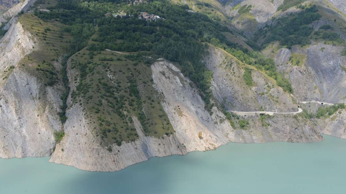
Fig. 6.1 View of the Chambon landslide (France) in July 2015 after the major rupture. The red arrow indicates the location of the TLS installed in front of the landslide.
Important
For a detailed information on Chambon landslide:
Desrues, M., Lacroix, P., & Brenguier, O. (2019). Satellite Pre-Failure Detection and In Situ Monitoring of the Landslide of the Tunnel du Chambon, French Alps. Geosciences, 9(7), 313. https://doi.org/10.3390/geosciences9070313
6.3.2. The Achoma landslide
The Achoma landslide Fig. 6.2 : is situated in the Colca valley in Peru which is a wide depression filled with lacustrine sediments deposited over the last 1Myr, after a major debris avalanche coming from the Hualca hualca volcanic complex damed the valley. After the breaching of the dam, Colca river started to incise the soft clayey sediments and initiated landsliding in the whole area. The Achoma landslide, of approximate size 500x500x80 m3 was triggered in June 2020, 2 months after the end of the rainy season. It destroyed cultures and blocked the Colca river, creating a lake, threatening the inhabitants downstream.
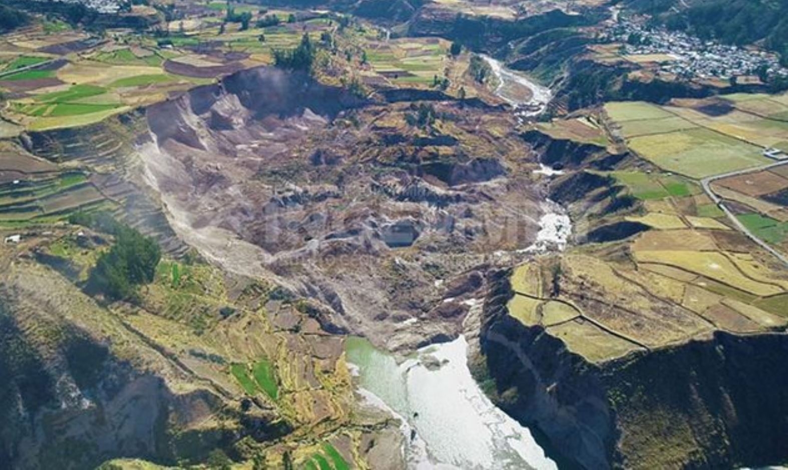
Fig. 6.2 View of the Achoma landslide (Peru) in August 2020 after its triggering.
Important
For a detailed information about landslides in Colca valley:
Zerathe, S., Lacroix, P., Jongmans, D., Marino, J., Taipe, E., Wathelet, M., Pari, W., Smoll, L. F., Norabuena, E., Guillier, B., and Tatard, L. (2016) Morphology, structure and kinematics of a rainfall controlled slow-moving Andean landslide, Peru. Earth Surf. Process. Landforms, 41: 1477–1493. doi: 10.1002/esp.3913.
6.4. Landslide occurrence time prediction
In this section, you will try to predict the occurrence time of the two landslides based on their latest phase of acceleration before rupture. For some landslides, that experience progressive maturation of faults, [27] found that the logarithm of the landslide acceleration (\(\ddot{\eta}\)) in its last stage before failure is proportional to the logarithm of its velocity (\(\dot{\eta}\)), i.e.:
Integrating this equations for a \(\alpha > 1\), one obtains:
In the specific case where \(\alpha = 2\), which is a close assumption for the tertiary creep of landslides, the equation reduces to the Saito Formula [28]:
This equation indicates that the time to failure \(t_f\) in tertiary creep is inversely proportional to the current strain rate or velocity. Plotting the inverse velocity of the landslide as a function of time therefore allows the estimation of the landslide failure, as represented in Figure 3.
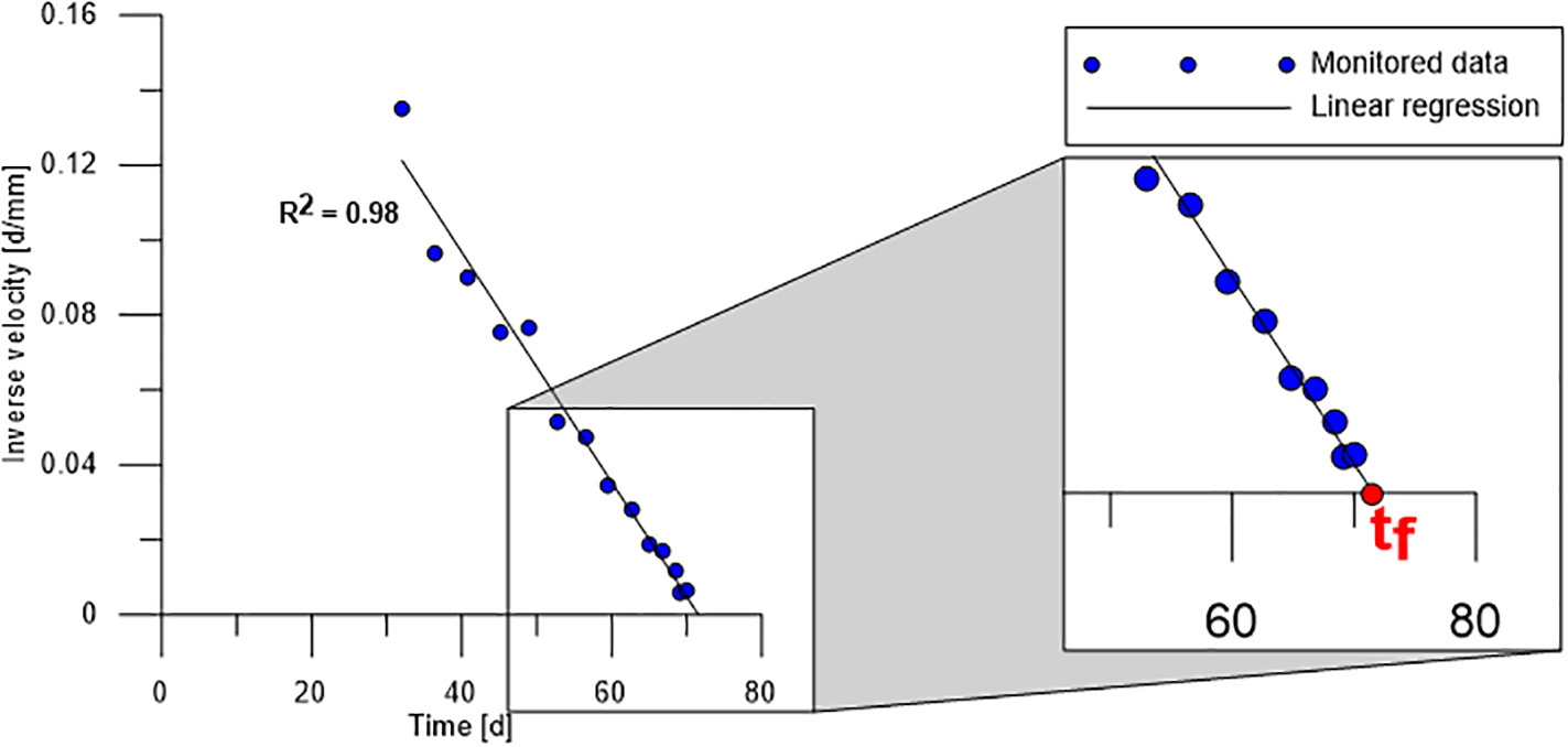
Fig. 6.3 Linear Fukuzono model application and the corresponding R² value, with a detail of the intersection between the linear regression and the x-axis. From [29].
Important
For a detailed information on the pre-failure landslide accelerations:
Federico, A., Popescu, M., Elia, G. et al. Prediction of time to slope failure: a general framework. Environ Earth Sci 66, 245–256 (2012). https://doi.org/10.1007/s12665-011-1231-5
6.5. Practical work
6.5.1. Chambon data
A network of 24 of topographic targets was set set up area in in June 2015 by the SAGE society Fig. 6.4. Seven targets were were located located in around the movement and 17 and on the unstable mass. Planimetric and altimetric displacements were regularly recorded thanks to an automatic theodolite placed in the southern side of the lake in front of the movement. The automatic theodolite placed in the southern side of the lake in front of the movement. The measurement frequency was 1.5 h with a precision of 2 mm, as estimated from the standard deviation calculated on targets located in the stable parts. For this practice you will use the data from the target C15.
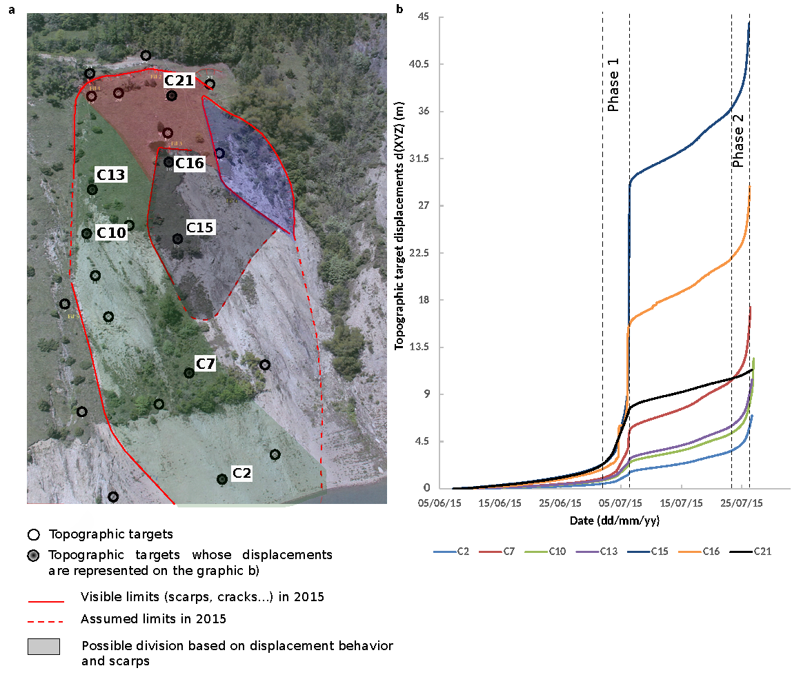
Fig. 6.4 Left: Position of the topographic targets on the Chambon landslide; Right: Cumlative displacements in meters of the selected topographic targets [26].
6.5.2. Achoma data
Year 2020 was one of the wettest rainy season from the last 30 years, that ended up in April 2020. Local inhabitants noted in June 2020 the existence of large fissures, but, after investigations from the Peruvian Geological office no monitoring was set up for different reasons, including the little risk posed to inhabitants (no habitations) and the lack of technical people to take charge of this monitoring during covid lowdown time. Therefore, the geodetical data analyzed in this practice comes from the reanalysis of remote-sensing images. Specifically from the correlation of Planet satellite images. Planet satellites enabled a quasi daily monitoring of the landslide with uncertainties of between 0.5 and 1 m. The interest of satellite images is the possibility of having spatially extended measurements. Here we selected only one point in the most rapid area.
6.6. Practice
6.6.1. Load the data
Important
For this practice, you will use Excel or LibreOffice to visualize the displacement as a function of the date as a scatter plot.
The data used in this exercise can be downloaded from:
6.6.2. Plot the data
Compute the landslide velocity using the Excel tools. Note the acceleration before the landslide failure.
Questions for discussion
Is the acceleration progressive?
When did it start?
6.6.3. Predict the time of failure
Based on the Fukuzono method [27], with \(\alpha = 2\) (Saito method [28], Fig. 6.3), applied on the progressively accelerating part of the displacement curve (see (6.3) in Section Landslide occurrence time prediction), predict the time-to-failure of each landslide. Reiterate this process by removing the last point(s) of the time-series before the failure. Draw the estimated date of your failure prediction as a function of your last measurements.
6.6.4. Discussion
Questions for discussion
How long in advance could have been predicted the landslide occurrence with a 1 day uncertainty? With a 2 day uncertainty? With a 1 week uncertainty
Discuss the pro and the cons of the satellite and in situ measurements?
Do you think satellite measurements could be used as a operational tool for landslide prediction?
How would you improve this approach for operational landslide risk management?
6.7. References
Joan A. Casey, Yuqian M. Gu, Lara Schwarz, Timothy B. Frankland, Lauren B. Wilner, Heather McBrien, Nina M. Flores, Arnab K. Dey, Gina S. Lee, Chen Chen, Tarik Benmarhnia, and Sara Y. Tartof. The 2025 Los Angeles Wildfires and Outpatient Acute Healthcare Utilization. medRxiv, pages 2025.03.13.25323617, March 2025. doi:10.1101/2025.03.13.25323617.
Jon E. Keeley and Alexandra D. Syphard. Large California wildfires: 2020 fires in historical context. Fire Ecology, 17(1):22, August 2021. doi:10.1186/s42408-021-00110-7.
Pascal Lacroix, Gael Araujo, James Hollingsworth, and Edu Taipe. Self-Entrainment Motion of a Slow-Moving Landslide Inferred From Landsat-8 Time Series. Journal of Geophysical Research: Earth Surface, 124(5):1201–1216, 2019. _eprint: https://agupubs.onlinelibrary.wiley.com/doi/pdf/10.1029/2018JF004920. URL: https://onlinelibrary.wiley.com/doi/abs/10.1029/2018JF004920 (visited on 2023-03-01), doi:10.1029/2018JF004920.
Laura Parra García, Gianluca Furano, Max Ghiglione, Valentina Zancan, Ernesto Imbembo, Christos Ilioudis, Carmine Clemente, and Paolo Trucco. Advancements in Onboard Processing of Synthetic Aperture Radar (SAR) Data: Enhancing Efficiency and Real-Time Capabilities. IEEE Journal of Selected Topics in Applied Earth Observations and Remote Sensing, 17:16625–16645, 2024. doi:10.1109/JSTARS.2024.3406155.
Diego Cusicanqui, Antoine Rabatel, Christian Vincent, Xavier Bodin, Emmanuel Thibert, and Bernard Francou. Interpretation of Volume and Flux Changes of the Laurichard Rock Glacier Between 1952 and 2019, French Alps. Journal of Geophysical Research: Earth Surface, 126(9):e2021JF006161, October 2021. doi:10.1029/2021JF006161.
Yifei Zhu, Xin Yao, Leihua Yao, and Chuangchuang Yao. Detection and characterization of active landslides with multisource SAR data and remote sensing in western Guizhou, China. Natural Hazards, 111(1):973–994, March 2022. doi:10.1007/s11069-021-05087-9.
Pascal Lacroix, Amaury Dehecq, and Edu Taipe. Irrigation-triggered landslides in a Peruvian desert caused by modern intensive farming. Nature Geoscience, 13(1):56–60, January 2020. Number: 1 Publisher: Nature Publishing Group. URL: https://www.nature.com/articles/s41561-019-0500-x (visited on 2023-03-01), doi:10.1038/s41561-019-0500-x.
David P. Roy, Haiyan Huang, Rasmus Houborg, and Vitor S. Martins. A global analysis of the temporal availability of PlanetScope high spatial resolution multi-spectral imagery. Remote Sensing of Environment, 264:112586, October 2021. doi:10.1016/j.rse.2021.112586.
Swann Zerathe, Pascal Lacroix, Denis Jongmans, Jersy Marino, Edu Taipe, Marc Wathelet, Walter Pari, Lionel Fidel Smoll, Edmundo Norabuena, Bertrand Guillier, and Lucile Tatard. Morphology, structure and kinematics of a rainfall controlled slow-moving Andean landslide, Peru. Earth Surface Processes and Landforms, 41(11):1477–1493, 2016. doi:10.1002/esp.3913.
Noélie Bontemps, Pascal Lacroix, and Marie-Pierre Doin. Inversion of deformation fields time-series from optical images, and application to the long term kinematics of slow-moving landslides in Peru. Remote Sensing of Environment, 210:144–158, June 2018. doi:10.1016/j.rse.2018.02.023.
Francois Ayoub, Sebastien Leprince, Renaud Binet, Kevin W. Lewis, Oded Aharonson, and Jean Philippe Avouac. Influence of camera distortions on satellite image registration and change detection applications: 2008 IEEE International Geoscience and Remote Sensing Symposium - Proceedings. 2008 IEEE International Geoscience and Remote Sensing Symposium - Proceedings, pages II1072–II1075, December 2008. doi:10.1109/IGARSS.2008.4779184.
Theodore A. Scambos, Melanie J. Dutkiewicz, Jeremy C. Wilson, and Robert A. Bindschadler. Application of image cross-correlation to the measurement of glacier velocity using satellite image data. Remote Sensing of Environment, 42(3):177–186, December 1992. doi:10.1016/0034-4257(92)90101-O.
Ross A. Beyer, Oleg Alexandrov, and Scott McMichael. The ames stereo pipeline: nasa's open source software for deriving and processing terrain data. Earth and Space Science, 5(9):537–548, 2018. doi:10.1029/2018EA000409.
David E. Shean, Oleg Alexandrov, Zachary M. Moratto, Benjamin E. Smith, Ian R. Joughin, Claire Porter, and Paul Morin. An automated, open-source pipeline for mass production of digital elevation models (dems) from very-high-resolution commercial stereo satellite imagery. ISPRS Journal of Photogrammetry and Remote Sensing, 116:101–117, 2016. doi:10.1016/j.isprsjprs.2016.03.012.
Diego Cusicanqui, Pascal Lacroix, Xavier Bodin, Benjamin Aubrey Robson, Andreas Kääb, and Shelley MacDonell. Detection and reconstruction of rock glacier kinematics over 24 years (2000–2024) from Landsat imagery. The Cryosphere, 19(7):2559–2581, July 2025. doi:10.5194/tc-19-2559-2025.
Martin Mergili, Adam Emmer, Anna Juřicová, Alejo Cochachin, Jan-Thomas Fischer, Christian Huggel, and Shiva P. Pudasaini. How well can we simulate complex hydro-geomorphic process chains? The 2012 multi-lake outburst flood in the Santa Cruz Valley (Cordillera Blanca, Perú). Earth Surface Processes and Landforms, 43(7):1373–1389, 2018. doi:10.1002/esp.4318.
I. Dussaillant, E. Berthier, F. Brun, M. Masiokas, R. Hugonnet, V. Favier, A. Rabatel, P. Pitte, and L. Ruiz. Two decades of glacier mass loss along the andes. Nature Geoscience, 12(10):802–808, 2019. doi:10.1038/s41561-019-0432-5.
D. Schneider, C. Huggel, A. Cochachin, S. Guillén, and J. García. Mapping hazards from glacier lake outburst floods based on modelling of process cascades at lake 513, carhuaz, peru. In Advances in Geosciences, volume 35, 145–155. 2014. URL: https://adgeo.copernicus.org/articles/35/145/2014/, doi:10.5194/adgeo-35-145-2014.
Diego Cusicanqui and Xavier Bodin. Photogrammetry for the study of mountain slopes. Webinar at INDURA, 2019. URL: https://vimeo.com/473376992.
Hideyuki Tonooka and Tetsushi Tachikawa. Aster cloud coverage assessment and mission operations analysis using terra/modis cloud mask products. Remote Sensing, 11(23):2798, 2019. doi:10.3390/rs11232798.
INAIGEM. Inventario nacional de glaciares y lagunas de origen glaciar 2023. Technical Report, Instituto Nacional de Investigación en Glaciares y Ecosistemas de Montaña, 2023. URL: https://hdl.handle.net/20.500.12748/499.
Romain Hugonnet, Robert McNabb, Etienne Berthier, Brian Menounos, Christopher Nuth, Luc Girod, Daniel Farinotti, Matthias Huss, Ines Dussaillant, Fanny Brun, and Andreas Kääb. Accelerated global glacier mass loss in the early twenty-first century. Nature, 592(7856):726–731, 2021. doi:10.1038/s41586-021-03436-z.
Fanny Brun, Etienne Berthier, Patrick Wagnon, Andreas Kääb, and Désirée Treichler. A spatially resolved estimate of high mountain asia glacier mass balances from 2000 to 2016. Nature Geoscience, 10(9):668–673, 2017. doi:10.1038/ngeo2999.
C. Nuth and A. Kääb. Co-registration and bias corrections of satellite elevation data sets for quantifying glacier thickness change. The Cryosphere, 5(1):271–290, March 2011. doi:10.5194/tc-5-271-2011.
A. Federico, M. Popescu, G. Elia, C. Fidelibus, G. Internò, and A. Murianni. Prediction of time to slope failure: a general framework. Environmental Earth Sciences, 66(1):245–256, May 2012. doi:10.1007/s12665-011-1231-5.
Mathilde Desrues, Pascal Lacroix, and Ombeline Brenguier. Satellite Pre-Failure Detection and In Situ Monitoring of the Landslide of the Tunnel du Chambon, French Alps. Geosciences, 9(7):313, July 2019. doi:10.3390/geosciences9070313.
Teruki Fukuzono. A new method for predicting the failure time of slope. In Proceedings, 4th Int'l. Conference and Field Workshop on Landslides, 145–150. 1985.
M Saito. Forecasting time of slope failure by tertiary creep. In Proceedings of 7th International Conference on Soil Mechanics and Foundation Engineering, 1969, volume 2, 677–683. 1969.
A. Segalini, A. Valletta, and A. Carri. Landslide time-of-failure forecast and alert threshold assessment: A generalized criterion. Engineering Geology, 245:72–80, November 2018. doi:10.1016/j.enggeo.2018.08.003.