3. Feature tracking image correlation
Diego CUSICANQUI1 & Pascal LACROIX1
1 Univ. Grenoble Alpes, CNES, CNRS, IRD, Institut des Sciences de la Terre (ISTerre), Grenoble, France.
Copyright
Document version 0.2, Last update: 2025-09-18
© PSF TelRIskNat 2025 Optical team (D. Cusicanqui, R. Basantes & P. Lacroix). This document and its contents are licensed under the Creative Commons Attribution 4.0 International License (CC BY-NC-SA 4.0).
3.1. Learning objectives:
Understand the principles of image correlation for measuring surface displacements.
Learn how to apply image correlation techniques using the ASP software.
Analyze and interpret displacement fields obtained from image correlation.
Note
This exercise focuses on optical remote sensing data from different sensors at different spatial resolution i.e. Planet (3m) or Sentinel2 (10m) or LandSat8 (15m). These remote sensing datasets have the greatest advantages of being free and available worldwide. For this practice, we will focus in the Maca Landslide in Peru using PlanetScope data.
3.2. INTRODUCTION
Landslides are a major threat in most mountainous areas of the world, causing nearly 10000 casualties every year. It has been observed that landslides can be preceded by a phase of acceleration, emphasising the interest in detecting slow ground-movements and monitoring their evolution through time. Knowing how the ground moves is essential to understanding the physical mechanisms controlling movement [3]. Landslide displacement can be measured from space by two techniques: first, by Interferometric Synthetic Aperture Radar (InSAR) and then, by feature-tracking image correlation applied either to SAR or optical images Fig. 3.1.
On one hand, surface deformation obtained from InSAR is now being used to measure very small displacements (e.g., < 1 cm) and detect new unstable zones. Although this technique offers the possibility to map very large areas (up to 400 km for Sentinel-1), this kind of data has a complex data processing and encounters different limitations related with the unwrapping of the signal that makes it not fully adapted to small objects like landslides or fast objects like glaciers [4]. On the other hand, optical image correlation is an appropriate technique for monitoring large displacements or long-term displacements of small objects [5]. Although freely available data exist worldwide (Section 2), the main limitations for this data are the presence of snow at the surface, clouds and strong changes in contrast caused by shadows. These two techniques have become the main means of studying natural hazards that produce deformations of the earth’s surface on different spatio-temporal scales [6].
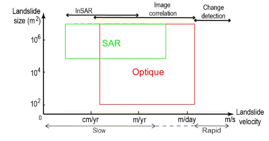
Fig. 3.1 Domain of applicability of different techniques and satellite data as a function of the landslide size and velocity [7] .
Note
In this practice, we will focus only on optical remote sensing data, at different resolutions.
3.3. REMOTE SENSING DATA
There are several possibilities to get freely available optical remote sensing data and many online services which offer access to the data worldwide. In this practice, we won’t cover all possible sources, but rather the most popular ones (i.e. Landsat 5/7/8, Sentinel-2 and Planet). For a comprehensive introduction you can see the Spatialpost <https://www.spatialpost.com/free-satellite-imagery/> webpage.
3.3.1. Landsat 4/5/7/8 legacy
The landsat program has been mapping earth since the early ~1970’s until now. Landsat satellites have continuously acquired space-based images of the Earth’s land surface, providing uninterrupted data to help land managers and policymakers make informed decisions about our natural resources and the environment. From a general point of view, this enormous dataset covers earth surface worldwide with a relatively medium spatial resolution 30 m and 15 m for multispectral and panchromatic bands, respectively. Landsat legacy has also a very good radiometric resolution between 5 to 11 bands depending on the landsat mission, as well as a good temporal resolution, one image each 16 days at equator and 2-3 days in the north pole. Landsat tiles cover a large spatial extent, with a 185 kilometres wide footprint. more information on USGS-landsat mission webpage.
Accessing LandSat7/8 data (Since 1999, 15m resolution, 16 days revisit time) could be possible though the following links:
3.3.2. Sentinel-2
The Copernicus SENTINEL-2 mission comprises a constellation of two polar-orbiting satellites placed in the same sun-synchronous orbit, phased at 180° to each other. It aims at monitoring variability in land surface conditions, and its wide swath width (290 km) and high revisit time (10 days at the equator with one satellite, and 5 days with 2 satellites under cloud-free conditions which results in 2-3 days at mid-latitudes) will support monitoring of Earth’s surface changes. More technical information though Copernicus Sentinel-2 program.
Accessing Sentinel-2 data (since December 2015, 10m resolution, 5 days revisit time) could be possible though the following links:
3.3.3. PlanetScope
PlanetScope, operated by Planet, is a constellation of approximately 130 satellites, able to image the entire land surface of the Earth every day (a daily collection capacity of 200 million km²/day, Fig. 3.2). PlanetScope images are approximately 3 metres per pixel resolution with 4 spectral bands Blue, Green, Red and IR bands. The data can be downloaded for free, within a certain quota, on the Planetscope website.
Accessing Planet data (Since ~2016, 3m resolution, ~1day revisit time):
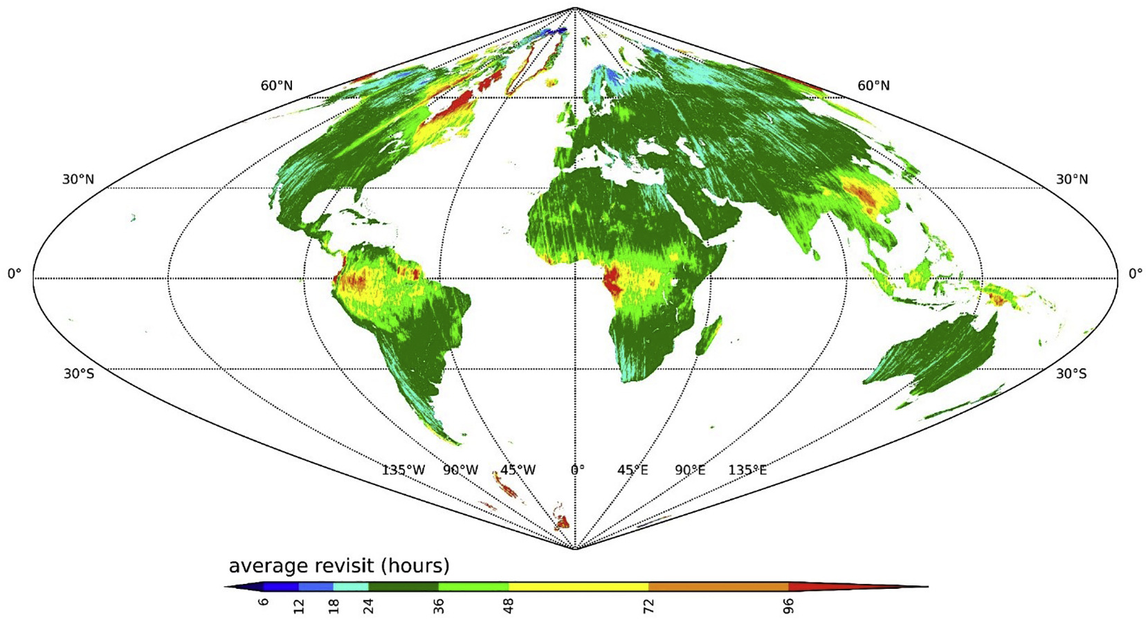
Fig. 3.2 Average revisit time between 2 Planet acquisitions (2019-2020), [8].
3.4. PRACTICE
3.4.1. About the study site - Maca Landslide, Peru
The Maca landslide Fig. 3.3 is situated in the Colca valley in Peru which is a wide depression filled with lacustrine sediments deposited over the last 1M yr, after a major debris avalanche coming from the “Hualca Hualca” volcanic complex dammed the valley. After the breaching of the dam, Colca river started to incise the soft clayey sediments and initiated landsliding in the whole area. Its historical activity can be traced back to the 1980’s, when the Lari landslide pushed the river down to the Maca side, and started to erode the Maca side. Several large reactivation occurred in 1990’s, 2000’s, 2012-2013, and 2019-2020 [3], [9], [10]. Examples for this practice will be taken during the last stage of reactivation, which produced major damages.
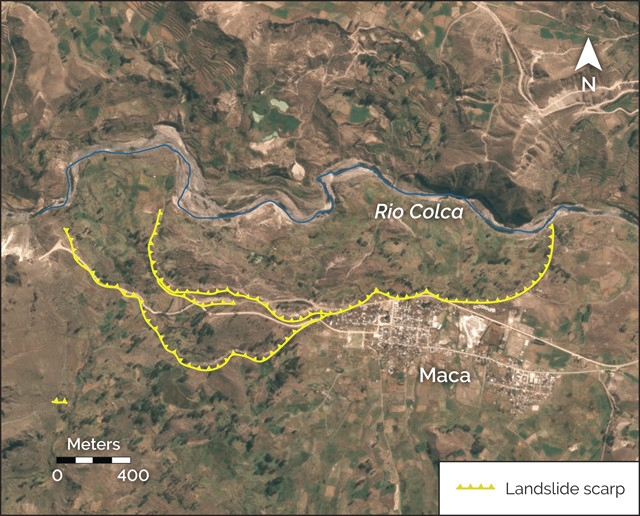
Fig. 3.3 Picture of the Maca landslide.
For this practice, landslide motion will be retrieved from correlation of optical images. The specific goal is to be able to produce maps such as the one shown in Fig. 3.4.
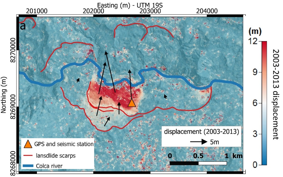
Fig. 3.4 Surface displacement field of the Maca landslide between 2003 and 2013 [10].
3.4.1.1. Download PlanetScope data
Log on the Planet server, select your area of interest (not too large, typically 4x3km, that includes the landslide and stable areas) and download at least 2 images (you can even select one per year 2017-2022), taken at the same season, without clouds. If possible select images that are not a mosaic of several images but only one single image. The image download is done with the “order scenes” blue button at the bottom left of the browser Fig. 3.5.
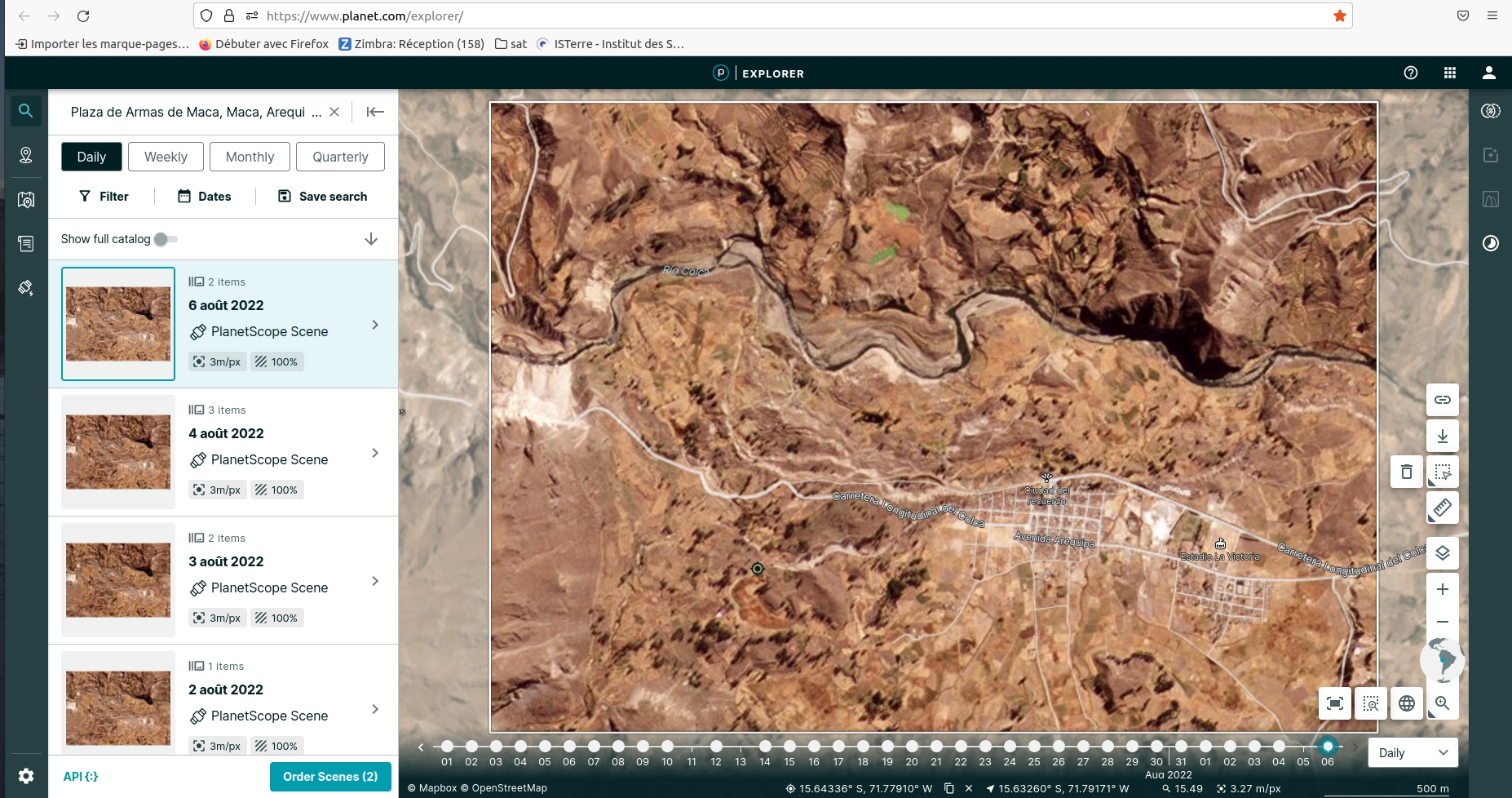
Fig. 3.5 Planet download interface centered on Maca landslide.
Note
Since the activation of the Planet account could take long-time, for this practice we already provide a set of images.
Now, open two images (those furthest back in time, 2018-2022). Open both images by clicking on Layer -> Add Raster Layer play with them by turning them on and off.
Questions for discussion
Can you tell if the landslide faced any changes during your period of study?
Are you able to track any displacement by eye?
3.4.2. About surface displacements and image correlation
Surface displacements are defined as the movement of the ground surface between two dates. They can be measured in different ways, either in-situ (e.g., GNSS, total station, extensometer, etc.) or remotely (e.g., optical or SAR image correlation, InSAR, LiDAR, etc.). In this practice we will focus on surface displacements measured from optical image correlation.
Surface displacements from image correlation are obtained by tracking the translation of small, textured pixel windows between two accurately co-registered, orthorectified images acquired at different dates. A similarity metric—typically normalized cross-correlation—yields sub-pixel offsets for each window; these offsets are converted to map-plane displacement vectors using pixel size. The method delivers dense 2-D horizontal motion fields (magnitude and direction), with uncertainty controlled by image texture, window size, co-registration accuracy, and radiometric changes [11]. The main principle of image correlation is to divide the first image into small windows (or chips) and then search for the best matching window in the second image. However, modern softwares have implemented different strategies and algorithms to improve the accuracy, robustness and speed of the correlation process.
Important
For the following exercise we will use two different algorithms to compute surface displacements: (1) IMCORR (SAGA-QGIS) and (2) ASP. We propose to compare both algorithms and discuss their advantages and limitations.
3.4.3. Compute surface displacements with IMCORR (SAGA-QGIS)
This first part of the exercise will be done using QGIS software with the SAGA plugin. This exercise can be done on any operating system (Windows, Linux or MacOS).
Important
Download a pair of Planet images (2018-2021) over the Maca landslide using this RENATER link.
Once images loaded in QGIS, we will use the SAGA plugin to compute surface displacements with the IMCORR algorithm. If you don’t have SAGA installed, please follow the instructions in the Installation of QGIS for data visualization (windows or linux independently) section of the installation guide.
Note
IMCORR algorithm is on of the first image correlation algorithms developed in the early 90’s [12]. It is now implemented in the SAGA GIS software and can be used through the QGIS interface. It has been widely used in glaciology to measure glacier surface displacements from optical images [12]. As this algorithm is no longer maintained, we will use only for academic purposes. It is therefore recommended to use more recent algorithms such as the one implemented in the ASP software (see Compute surface displacements with ASP).
3.4.3.1. Prepare the images
IMCORR algorithm accepts single band images with the same number of columns (width) and lines (height). So, you will need to first extract the red band (band 3) from both Planet images and then clip them to the same extent. As this is a common processing step, we wont detail it here.
Tip
For extract single band, you can use
GDAL -> Raster conversion -> Rearange bandswithin QGIS.For clipping images you can use the
Clip Raster by Extenttool in QGIS to clip both images to the same extent. Make sure to check the optionUse Layer Extentand select one of your two images as the layer to define the extent.You can check the number of columns and lines of your images by right-clicking on the layer and selecting
Properties -> Informationtab.
3.4.3.2. Image correlation and outputs
Now, in the Processing Toolbox of QGIS, search for IMCORR and open the Image Correlation (IMCORR) tool. Fill the parameters as Fig. 3.6 and run the tool.
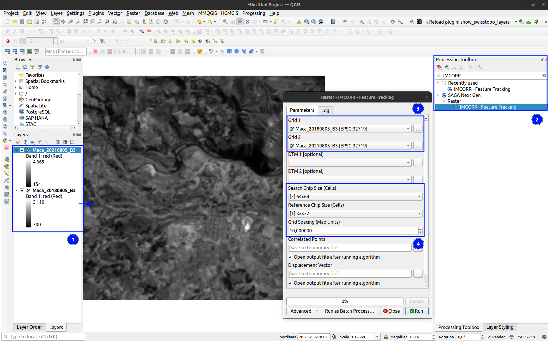
Fig. 3.6
IMCORR parameters in QGIS. 1 and 3) Input images (single band, same size), 2) IMCORR algorithm, 4) Correlation parameters (Search chip size, Reference chip size, Grid spacing).
Important
The choice of the parameters is crucial to obtain good results. Here are some advices:
search chip size (pixels): Chip size of search chip, used to find correlating reference chips in the second image. A larger chip size will increase the chance of finding a match, but will also increase computation time. A typical value is 64x64 pixels.
reference chip size (pixels): Chip size of reference chip to be found in search chip. used to find correlating search chips in the first image. A larger chip size will increase the chance of finding a match, but will also increase computation time. A typical value is 32x32 pixels. This parameter can be equal or less to the search chip size.
Grid spacing (Map units): Spacing between grid points where displacements are calculated. A smaller spacing will give a more detailed displacement field, but will also increase computation time. A typical value is 10 pixels.
The output of the IMCORR tool are two vector files: Correlated points and Displacement vectors. You can load them in QGIS and visualize them as Fig. 3.7.
The
Correlated pointslayer contains all details about the correlation process (i.e. displacemets along columns (EW) and rows (NS), correlation coefficient, pixel coordinates, displacement in pixels, etc) for each grid point Fig. 3.7.The
Displacement vectorslayer contains only the displacement vectors for each grid point oriented though the direction of the displacement. THe lenght of the vectors is proportional to the displacement amplitude Fig. 3.7.
Within the correlated points, you can visualize the DISP column that contains the total displacement amplitude (in meters) for each grid point Fig. 3.7. You can also visualize the STRENGTH column that contains how the correlation is between pixels (greater values means better correlation). In addition to these two important columns, you can also visualize the XERR and YERR columns that contain the uncertainty of the displacement along columns (EW) and rows (NS), respectively.
Tip
You can filter the correlated points by the STRENGTH, DISP, XERR and YERR columns to keep only the best correlated points (e.g. STRENGTH > 6 or 2 pixels) or those points with low uncertainty (e.g. XERR < 1 or YERR < 1) Fig. 3.7.
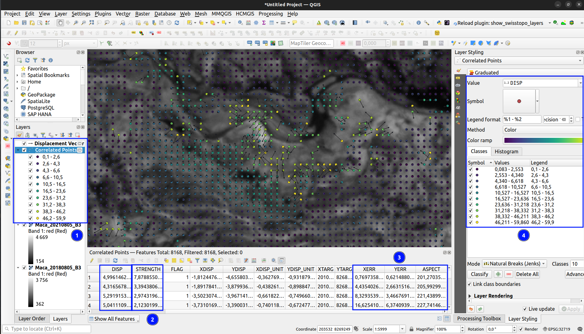
Fig. 3.7
IMCORR outputs in QGIS: 1) Correlated points and Displacement vectors layers. 2) and 3) Important outputs within the Correlated points layer, 4) Correlation points coloured by displacements (DISP column). Background image corresponds to Maca landslide in Planet 2021 image.
3.4.3.3. Interpolation of surface displacements
To visualize the displacement field as a raster, you can interpolate the DISP column of the Correlated points layer using the IDW interpolation or Heatmap tool in QGIS. You can also interpolate the DX and DY columns to obtain the displacement along columns (EW) and rows (NS), respectively. The result should be similar to Fig. 3.8.
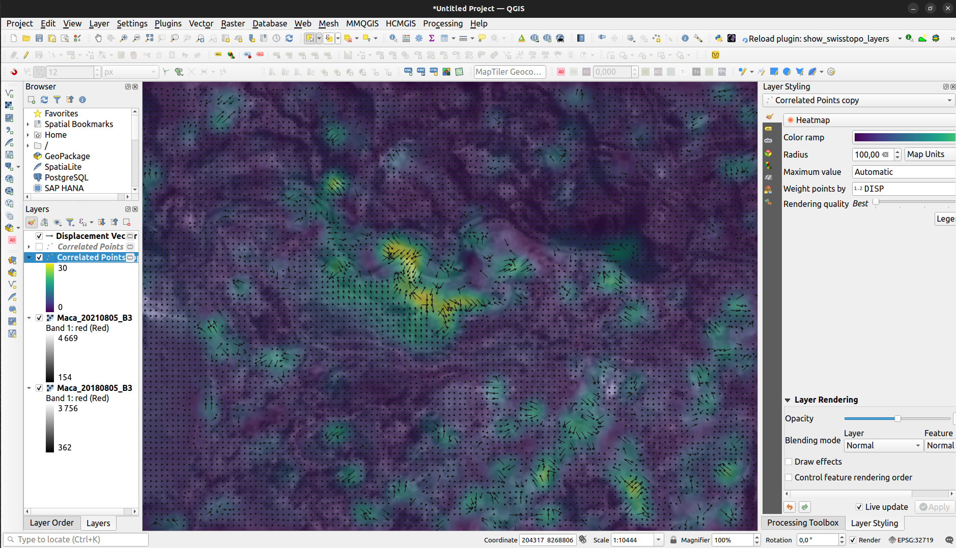
Fig. 3.8
Interpolation of the DISP column of the Correlated points layer using the Heatmap tool in QGIS. Background image corresponds to Maca landslide in Planet 2021 image.
Questions for discussion
What do you think of the results obtained with IMCORR?
What are the main patterns of displacement that you can observe?
What do you think about the noise-level of the displacement field?
What are the main sources of errors?
What are the advantages and limitations of the IMCORR algorithm?
How would you improve the results obtained with IMCORR?
3.4.4. Compute surface displacements with ASP
To measure surface displacements field using Ames Stereo Pipeline (ASP), you will use the different correlator strategies developed in the ASP software. Among them, the classic Block Matching (BM) algorithm and the Normalised Cross Correlation (NCC) cost-function (for correlation quality) are the most commonly used. The process initially requires 2 images as main input data. However, there is several parameters that can be tuned to improve the quality of the results. For instance, the size of the correlation window (or kernel), the type of correlation algorithm (BM, Semi-Global Matching (SGM), etc), the refinement of the correlation function (subpixel-mode). In this practice, we will use the parallel_stereo command to compute the displacement fields and the corr_eval command to compute a quality metric (NCC) of the correlation process.
The window size is fixed to 21x21. It can be tuned by using the option –corr-kernel. Other parameters, like the type of correlation algorithm or the refinement of the correlation function, can also be tuned. For instance the refinement mode 2 (Bayes mode) is the slowest one, but also the most precise. If you want a more rapid evaluation of your displacement fields, use subpixel-mode 1 (parabola fitting).
See also
Ames Stereo Pipeline (ASP) The NASA Ames Stereo Pipeline (ASP) is an open-source photogrammetric software, to generate DEM from either multiple satellite, airborne or ground-based images on the Earth and other planetary bodies (Mars, Moon, etc). This software is designed to produce DEM’s using stereo or multiple-stereo pairs of optical images. For more detailed and complete information please refer to NASA ASP web page. Read on Ames Stereo Pipeline: [13] & [14].
3.4.4.1. Download the data
This second part of the exercise will be done using ASP software. This exercise will be run on Linux (e.g. WSL or Virtual Machine) or MAC operating system.
Important
Download a set of Planet images (2018-2025) over the Maca landslide. You can use the provided script located in /psf_telrisknat_2025_docs/data/download_excercise_2_data.sh as follow:
Open a terminal and navigate to the
/psf_telrisknat_2025_docs/data/directory.
cd ~/psf_telrisknat_2025_docs/data/
Run the following command:
bash download_excercise_2_data.sh
3.4.4.2. Prepare the images
As for IMCORR, ASP requires single band images with the same number of columns (width) and lines (height). So, you will need to first extract the red band (band 3) from both Planet images and then clip them to the same extent. As we provide the data ready for processing, we wont provide the details here:
gdal_translate -of GTiff -co COMPRESS=None -co NBITS=16 \
-b 3 <image-input.tif> <image-output-B3.tif>
3.4.4.3. Image correlation using parallel_stereo
Now, you can run the parallel_stereo command with the following parameters:
parallel_stereo --correlator-mode --stereo-algorithm asp_bm --subpixel-mode 2 \
--threads 16 --corr-kernel 21 21 \
Maca_20180805_B3.tif Maca_20210805_B3.tif run/run-corr-20180805-20210805
The output directory run contains run-corr-20180805-20210805-F.tif (3 bands):
Band 1: EW (column) displacement (pixels)
Band 2: NS (row) displacement (pixels)
Band 3: GoodPixelMap (raster mask of valid pixels)
3.4.4.4. Quality metric (NCC)
To evaluate the quality of the correlation process, estimated by the cross-correlation coefficient (CC), you must run the following command:
corr_eval --kernel-size 21 21 --metric ncc --prefilter-mode 2 --threads 16 \
Maca_20180805_B3.tif Maca_20210805_B3.tif run/run-corr-20180805-20210805-F.tif run/run-corr-20180805-20210805
This comand creates a raster file named run/run-corr-20180805-20210805-ncc.tif with values in [0, 1]. The NCC files contain a raster where their values are coded between 0 and 1, where values close to 0 have low correlation and values close to 1 have good correlation.
3.4.4.5. Harmonizing data for better analysis and visualization
Now you will separate first band and second, which corresponds to EW and NS. Run the following commands:
gdal_translate -of GTiff -co COMPRESS=None -co NBITS=16 -b 1 \
run/run-corr-20180805-20210805-F.tif EW_20180805_20210805.tif
gdal_translate -of GTiff -co COMPRESS=None -co NBITS=16 -b 2 \
run/run-corr-20180805-20210805-F.tif NS_20180805_20210805.tif
mv run/run-corr-20180805-20210805-ncc.tif CC_20180805_20210805.tif
3.4.4.6. Convert from pixels to metres
Note that contrary to IMCORR algorithm, ASP provides surface displacement in pixels. To convert it into meters, you must multiply by the pixel resolution (in this case 3m). You can use the raster calculator of QGIS to do so, or directly with the gdal library. Run the following commands:
gdal_calc.py -A EW_20180805_20210805.tif --outfile=EWm_20180805_20210805.tif --calc="A*3"
gdal_calc.py -A NS_20180805_20210805.tif --outfile=NSm_20180805_20210805.tif --calc="A*-3"
Once the results are converted, you can use QGIS environments to visualise the results :Fig. 3.9.
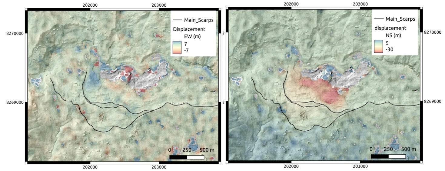
Fig. 3.9
ASP outputs in QGIS: Left: EWm_20180805_20210805.tif, Right: NSm_20180805_20210805.tif. Background image corresponds to Maca landslide hillshade.
We will now compute the total displacement field (See (3.1)). For that, we will use the output of the previous results using the following formula:
where d is magnitude displacements in meters, NSm is raster displacements of the North-Sud component in meters, EWm is raster displacements of the East-West component in meters.
You can use the raster calculator of QGIS to do so, or directly with the gdal library. Run the following command:
gdal_calc.py -A EWm_20180805_20210805.tif -B NSm_20180805_20210805.tif \
--outfile=DISPm_20180805_20210805.tif --calc="sqrt(A**2 + B**2)"
Questions for discussion
Load the EW_20180805_20210805.tif, NS_20180805_20210805.tif and CC_20180805_20210805.tif files in QGIS to visualize them.
What do you think of the results obtained with ASP?
What are the main patterns of displacement that you can observe?
What do you think about the noise-level of the displacement field?
What are the main sources of errors?
What are the advantages and limitations of the ASP algorithm?
3.4.4.7. Bias correction in surface displacements
When inspecting the images in QGIS, you may notice that two of them are not perfectly georeferenced due to gyroscope errors on the satellite. There may be a bias of up to 10 m between them. This bias is clearly visible in stable areas where motion should be close to zero. However, as can be seen in Fig. 3.9, this is not the case. To remove this bias, we need to visualise the east-west (EW) and north-south (NS) histograms in QGIS Fig. 3.10, evaluate the value at the peak and subtract it separately for the EW and NS bands.
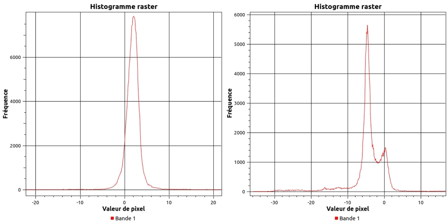
Fig. 3.10
Surface displacement histograms in QGIS: Left: EWm_20180805_20210805.tif, Right: NSm_20180805_20210805.tif.
In order to correct this bias, you can use either the raster calculator in QGIS or directly with the gdal library to do this subtraction. Run the following commands:
gdal_calc.py -A EWm_20180805_20210805.tif --outfile=EWm_20180805_20210805_bc.tif --calc="A-2.0"
gdal_calc.py -A NSm_20180805_20210805.tif --outfile=NSm_20180805_20210805_bc.tif --calc="A+4.6"
Finally, you can compute the total displacement and surface velocity as follows:
gdal_calc.py -A EWm_20180805_20210805_bc.tif -B NSm_20180805_20210805_bc.tif \
--outfile=DISPm_20180805_20210805_bc.tif --calc="sqrt(A**2 + B**2)"
Visualize the displacement field overlayed over a hillshade DEM (if you have one, either over the satellite image in B&W). Adjust the transparency of the displacement layer right-clicking on the layer -> Properties. The results should be similar to Fig. 3.11.
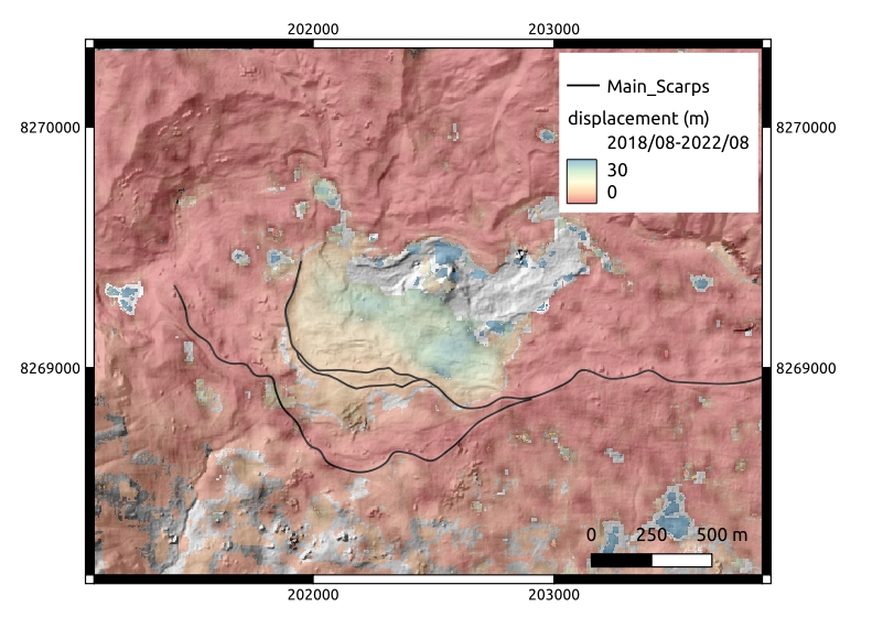
Fig. 3.11
ASP bias corrected outputs in QGIS: DISPm_20180805_20210805_bc.tif. Background image corresponds to Maca landslide hillshade.
Tip
ASP do not provide the displacement vectors as IMCORR. However, you can create them in QGIS. Take a look at this tutorial.
Questions for discussion
Load the DISPm_20180805_20210805.tif and DISPm_20180805_20210805_bc.tif files in QGIS and compare them.
What do you think of the results obtained with ASP after bias correction?
What are the main patterns of displacement that you can observe?
What do you think about the noise-level of the displacement field?
What are the main sources of errors?
What are the advantages and limitations of the ASP algorithm?
3.4.5. Evaluation of the data quality
Once you have obtained the displacement fields with both IMCORR and ASP (or any other algorithm), the questions is How to evaluate the data quality?
Some aspects to consider include:
Tip
Comparison with ground truth data: If available, compare the displacement fields with in-situ measurements or other reliable data sources to assess accuracy. For instance on the Maca landslide, 3 permanent GNSS enabled this comparison Fig. 3.12. This point-to-point evaluation allows us to give confidence to feature tracking results.
Statistical analysis: Calculate statistics such as mean, median, standard deviation, and interquartile range to quantify the displacement field characteristics. This can be done using stable areas where no displacement is expected (e.g., areas with no known ground movement [15]). However, you should pay attention on how those stable areas are defined.
Uncertainty estimation: Assess the uncertainty associated with the displacement measurements, which can be influenced by factors such as image resolution, correlation window size, and image quality. For instance a standard deviation (STD) of the EW and NS measurements component on a stable area can be used to evaluate the uncertainties.
Visual inspection: Look for obvious errors, such as unrealistic displacements or patterns that do not make sense given the context of the study area.
Cross-validation: If multiple displacement fields are available (e.g., from different algorithms or time periods), compare them to identify consistent patterns and potential biases.
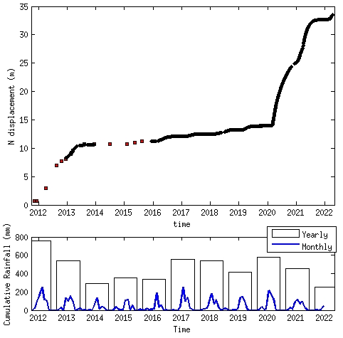
Fig. 3.12 Example of data quality evaluation using in-situ GNSS data on the Maca landslide [7]. Time-series of displacement measured by a GNSS installed on the Maca landslide.
3.5. To go further
Important
Do it yourself!!
Congratulations!! Now you have the basic knowledge on how to compute surface displacement using both IMCORR algorithm in QGIS and ASP. To go further:
Replicate the same process using other PlanetScope pair images available in the directory
data/excercice_2_image_correlation/maca_planet. For instance, you can use the 2021-2025 pair.
3.6. References
Joan A. Casey, Yuqian M. Gu, Lara Schwarz, Timothy B. Frankland, Lauren B. Wilner, Heather McBrien, Nina M. Flores, Arnab K. Dey, Gina S. Lee, Chen Chen, Tarik Benmarhnia, and Sara Y. Tartof. The 2025 Los Angeles Wildfires and Outpatient Acute Healthcare Utilization. medRxiv, pages 2025.03.13.25323617, March 2025. doi:10.1101/2025.03.13.25323617.
Jon E. Keeley and Alexandra D. Syphard. Large California wildfires: 2020 fires in historical context. Fire Ecology, 17(1):22, August 2021. doi:10.1186/s42408-021-00110-7.
Pascal Lacroix, Gael Araujo, James Hollingsworth, and Edu Taipe. Self-Entrainment Motion of a Slow-Moving Landslide Inferred From Landsat-8 Time Series. Journal of Geophysical Research: Earth Surface, 124(5):1201–1216, 2019. _eprint: https://agupubs.onlinelibrary.wiley.com/doi/pdf/10.1029/2018JF004920. URL: https://onlinelibrary.wiley.com/doi/abs/10.1029/2018JF004920 (visited on 2023-03-01), doi:10.1029/2018JF004920.
Laura Parra García, Gianluca Furano, Max Ghiglione, Valentina Zancan, Ernesto Imbembo, Christos Ilioudis, Carmine Clemente, and Paolo Trucco. Advancements in Onboard Processing of Synthetic Aperture Radar (SAR) Data: Enhancing Efficiency and Real-Time Capabilities. IEEE Journal of Selected Topics in Applied Earth Observations and Remote Sensing, 17:16625–16645, 2024. doi:10.1109/JSTARS.2024.3406155.
Diego Cusicanqui, Antoine Rabatel, Christian Vincent, Xavier Bodin, Emmanuel Thibert, and Bernard Francou. Interpretation of Volume and Flux Changes of the Laurichard Rock Glacier Between 1952 and 2019, French Alps. Journal of Geophysical Research: Earth Surface, 126(9):e2021JF006161, October 2021. doi:10.1029/2021JF006161.
Yifei Zhu, Xin Yao, Leihua Yao, and Chuangchuang Yao. Detection and characterization of active landslides with multisource SAR data and remote sensing in western Guizhou, China. Natural Hazards, 111(1):973–994, March 2022. doi:10.1007/s11069-021-05087-9.
Pascal Lacroix, Amaury Dehecq, and Edu Taipe. Irrigation-triggered landslides in a Peruvian desert caused by modern intensive farming. Nature Geoscience, 13(1):56–60, January 2020. Number: 1 Publisher: Nature Publishing Group. URL: https://www.nature.com/articles/s41561-019-0500-x (visited on 2023-03-01), doi:10.1038/s41561-019-0500-x.
David P. Roy, Haiyan Huang, Rasmus Houborg, and Vitor S. Martins. A global analysis of the temporal availability of PlanetScope high spatial resolution multi-spectral imagery. Remote Sensing of Environment, 264:112586, October 2021. doi:10.1016/j.rse.2021.112586.
Swann Zerathe, Pascal Lacroix, Denis Jongmans, Jersy Marino, Edu Taipe, Marc Wathelet, Walter Pari, Lionel Fidel Smoll, Edmundo Norabuena, Bertrand Guillier, and Lucile Tatard. Morphology, structure and kinematics of a rainfall controlled slow-moving Andean landslide, Peru. Earth Surface Processes and Landforms, 41(11):1477–1493, 2016. doi:10.1002/esp.3913.
Noélie Bontemps, Pascal Lacroix, and Marie-Pierre Doin. Inversion of deformation fields time-series from optical images, and application to the long term kinematics of slow-moving landslides in Peru. Remote Sensing of Environment, 210:144–158, June 2018. doi:10.1016/j.rse.2018.02.023.
Francois Ayoub, Sebastien Leprince, Renaud Binet, Kevin W. Lewis, Oded Aharonson, and Jean Philippe Avouac. Influence of camera distortions on satellite image registration and change detection applications: 2008 IEEE International Geoscience and Remote Sensing Symposium - Proceedings. 2008 IEEE International Geoscience and Remote Sensing Symposium - Proceedings, pages II1072–II1075, December 2008. doi:10.1109/IGARSS.2008.4779184.
Theodore A. Scambos, Melanie J. Dutkiewicz, Jeremy C. Wilson, and Robert A. Bindschadler. Application of image cross-correlation to the measurement of glacier velocity using satellite image data. Remote Sensing of Environment, 42(3):177–186, December 1992. doi:10.1016/0034-4257(92)90101-O.
Ross A. Beyer, Oleg Alexandrov, and Scott McMichael. The ames stereo pipeline: nasa's open source software for deriving and processing terrain data. Earth and Space Science, 5(9):537–548, 2018. doi:10.1029/2018EA000409.
David E. Shean, Oleg Alexandrov, Zachary M. Moratto, Benjamin E. Smith, Ian R. Joughin, Claire Porter, and Paul Morin. An automated, open-source pipeline for mass production of digital elevation models (dems) from very-high-resolution commercial stereo satellite imagery. ISPRS Journal of Photogrammetry and Remote Sensing, 116:101–117, 2016. doi:10.1016/j.isprsjprs.2016.03.012.
Diego Cusicanqui, Pascal Lacroix, Xavier Bodin, Benjamin Aubrey Robson, Andreas Kääb, and Shelley MacDonell. Detection and reconstruction of rock glacier kinematics over 24 years (2000–2024) from Landsat imagery. The Cryosphere, 19(7):2559–2581, July 2025. doi:10.5194/tc-19-2559-2025.
Martin Mergili, Adam Emmer, Anna Juřicová, Alejo Cochachin, Jan-Thomas Fischer, Christian Huggel, and Shiva P. Pudasaini. How well can we simulate complex hydro-geomorphic process chains? The 2012 multi-lake outburst flood in the Santa Cruz Valley (Cordillera Blanca, Perú). Earth Surface Processes and Landforms, 43(7):1373–1389, 2018. doi:10.1002/esp.4318.
I. Dussaillant, E. Berthier, F. Brun, M. Masiokas, R. Hugonnet, V. Favier, A. Rabatel, P. Pitte, and L. Ruiz. Two decades of glacier mass loss along the andes. Nature Geoscience, 12(10):802–808, 2019. doi:10.1038/s41561-019-0432-5.
D. Schneider, C. Huggel, A. Cochachin, S. Guillén, and J. García. Mapping hazards from glacier lake outburst floods based on modelling of process cascades at lake 513, carhuaz, peru. In Advances in Geosciences, volume 35, 145–155. 2014. URL: https://adgeo.copernicus.org/articles/35/145/2014/, doi:10.5194/adgeo-35-145-2014.
Diego Cusicanqui and Xavier Bodin. Photogrammetry for the study of mountain slopes. Webinar at INDURA, 2019. URL: https://vimeo.com/473376992.
Hideyuki Tonooka and Tetsushi Tachikawa. Aster cloud coverage assessment and mission operations analysis using terra/modis cloud mask products. Remote Sensing, 11(23):2798, 2019. doi:10.3390/rs11232798.
INAIGEM. Inventario nacional de glaciares y lagunas de origen glaciar 2023. Technical Report, Instituto Nacional de Investigación en Glaciares y Ecosistemas de Montaña, 2023. URL: https://hdl.handle.net/20.500.12748/499.
Romain Hugonnet, Robert McNabb, Etienne Berthier, Brian Menounos, Christopher Nuth, Luc Girod, Daniel Farinotti, Matthias Huss, Ines Dussaillant, Fanny Brun, and Andreas Kääb. Accelerated global glacier mass loss in the early twenty-first century. Nature, 592(7856):726–731, 2021. doi:10.1038/s41586-021-03436-z.
Fanny Brun, Etienne Berthier, Patrick Wagnon, Andreas Kääb, and Désirée Treichler. A spatially resolved estimate of high mountain asia glacier mass balances from 2000 to 2016. Nature Geoscience, 10(9):668–673, 2017. doi:10.1038/ngeo2999.
C. Nuth and A. Kääb. Co-registration and bias corrections of satellite elevation data sets for quantifying glacier thickness change. The Cryosphere, 5(1):271–290, March 2011. doi:10.5194/tc-5-271-2011.
A. Federico, M. Popescu, G. Elia, C. Fidelibus, G. Internò, and A. Murianni. Prediction of time to slope failure: a general framework. Environmental Earth Sciences, 66(1):245–256, May 2012. doi:10.1007/s12665-011-1231-5.
Mathilde Desrues, Pascal Lacroix, and Ombeline Brenguier. Satellite Pre-Failure Detection and In Situ Monitoring of the Landslide of the Tunnel du Chambon, French Alps. Geosciences, 9(7):313, July 2019. doi:10.3390/geosciences9070313.
Teruki Fukuzono. A new method for predicting the failure time of slope. In Proceedings, 4th Int'l. Conference and Field Workshop on Landslides, 145–150. 1985.
M Saito. Forecasting time of slope failure by tertiary creep. In Proceedings of 7th International Conference on Soil Mechanics and Foundation Engineering, 1969, volume 2, 677–683. 1969.
A. Segalini, A. Valletta, and A. Carri. Landslide time-of-failure forecast and alert threshold assessment: A generalized criterion. Engineering Geology, 245:72–80, November 2018. doi:10.1016/j.enggeo.2018.08.003.