5. Manual and automatic DEM co-registration
Diego CUSICANQUI1 & Ruben BASANTES2
1 Univ. Grenoble Alpes, CNES, CNRS, IRD, Institut des Sciences de la Terre (ISTerre), Grenoble, France.
2 Universidad Yachay Tech, Escuela de Ciencias de la Tierra, Energía y Ambiente, San Miguel de Urcuquí, Ecuador
Copyright
Document version 0.2, Last update: 2025-09-18
© PSF TelRIskNat 2025 Optical team (D. Cusicanqui, R. Basantes & P. Lacroix). This document and its contents are licensed under the Creative Commons Attribution 4.0 International License (CC BY-NC-SA 4.0).
5.1. Learning objectives:
Understand the principles of co-registration technique.
Learn how to apply image co-registration techniques manually and automatically.
Note
For this practice, you will use ASTER derived DEMs produced during the practice of Automatic generation of Digital Elevation Models using ASTER images to study the region of Cordillera Blanca
5.2. Introduction
As mentioned previously in the practice Automatic generation of Digital Elevation Models using ASTER images, quantification of mass changes is crucial to understand the fundamental processes that trigger mass-wasting events. Thus, a comparison of two or more 3D surfaces (e.g. Digital Elevation Models) could help to quantify these mass changes. However, DEM quality is highly dependent on several parameters, such as camera resolution, height flight, image quality, percentage of stereo coverage, etc., which play a major role in the quality of the DEMs and how they represent the 3D relief. Nowadays, there are several tools to generate DEMs, most of them in an automatic way. Because DEMs are the primary source for mass changes estimations, it is very important to assess the quality of DEMs, to avoid misinterpretations on the results.
During the automatic DEM generation, there are several sources of error that can affect the final DEM, for example translation and/or rational displacements on the spatial reference, as well as scale variations. In this practice, you will focus on the co-registration procedure used to adjust geometrically a pair of a DEMs. This method fits all DEMs regardless of the technique by which they were generated. For our example, we will use two DEMs automatically generated from ASTER optical images acquired on two different dates. After a brief description of the theoretical basis of the methodology, you will carry on in two hands-on co-registering exercises, the first based on an excel worksheet that will help you understand how the co-registering works, and the second will teach you how you can automate the co-registration procedure based on the application of Python libraries.
5.3. About DEM co-registration
Based on the results of the practice Compute difference of DEMs (DoD), you may notice that all east- and northeast (southwest)-facing slopes have strong positive (negative) differences in surface elevation Fig. 5.1. This indicates some kind of systematic bias between the two DEMs used to calculate the DEM difference. This type of bias is usually due to slight horizontal (EW or NS) and vertical shifts in one or both of the DEMs Fig. 5.1, which cause misleading elevation changes, especially on steep slopes where you can have strong elevation differences in a few meters. In short, this means that the DEMs are spatially inconsistent.
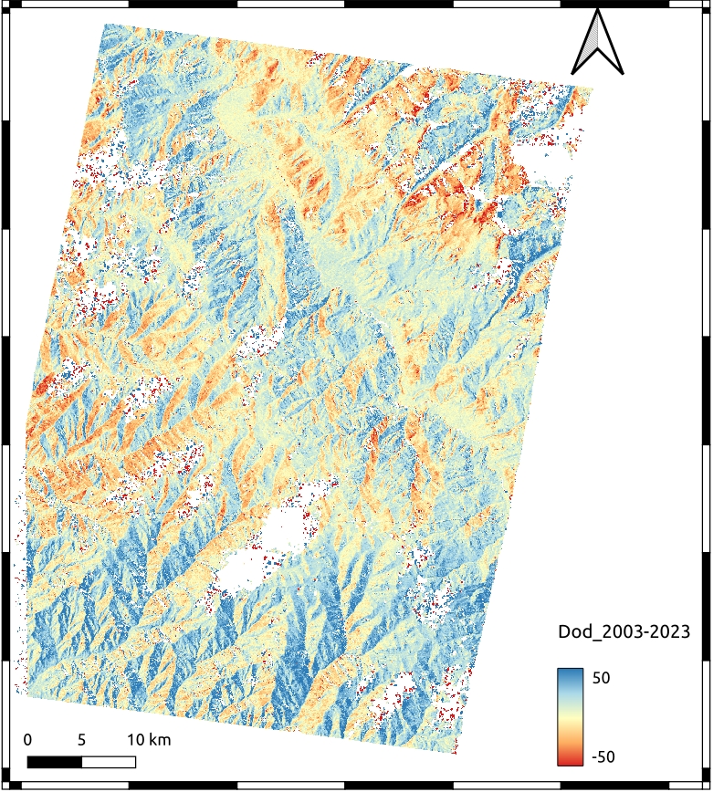
Fig. 5.1 Difference of DEMs (DoD) generated from ASTER images using ASP between 2003 and 2023. Visualized in QGIS.
To ensure a precise xyz alignment between the DEMs, an iterative method called co-registration proposed by [24] is commonly applied. This method is based on the elevation differences of the two misaligned DEMs, and it assumes that the surface elevation change is a function of the slope and the aspect of the terrain :numref:``.
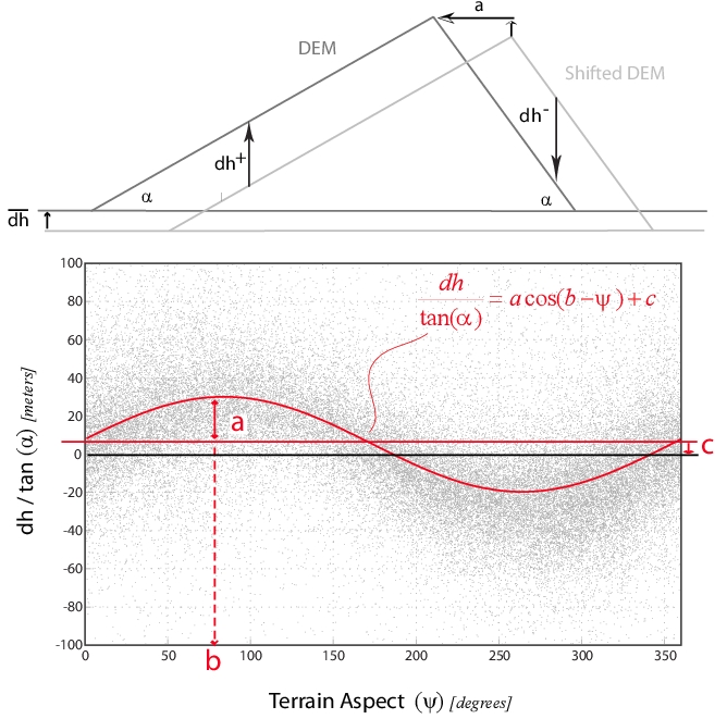
Fig. 5.2 Systematic bias in elevation due to slight shifts in one or both DEMs (from [24]).
This 3D spatial correction takes the most accurate DEM as a geodetic reference, whereas the second DEM is compared with the reference and co-registered (i.e. shifted) according the follow relationship:
where a is the magnitude of the misalignment, b is the direction of the misalignment, and c is the mean elevation bias. Then, the adjustment factors are computed as follow:
where Δx, Δy, and Δz are the horizontal (East-West and North-South) and vertical shifts, respectively, and \bar{\alpha} is the mean slope of the terrain. The process is repeated iteratively until the adjustment factors converge to zero (i.e., no further improvement in the alignment). The method assumes that the horizontal shifts are small compared to the pixel size of the DEMs, and that there are no significant elevation changes between the two acquisition dates.
Important
For a detailed explanation of the method:
Nuth, C. and Kääb, A. (2011): Co-registration and bias corrections of satellite elevation data sets for quantifying glacier thickness change, The Cryosphere, 5, 271-290, https://doi.org/10.5194/tc-5-271-2011.
5.4. Practice
5.4.1. Manual co-registration
5.4.1.1. Data inspection
For the first part of the exercise, you will use QGIS and Excel as the main softwares. This practice should be done in a computer with Windows OS.
Important
Download the data provided for this practice here Download data exercise 4.
First of all, you will open the DoD 2023-2003.tif Fig. 5.1 into QGIS and you will explore the data by looking at the histogram values of the DoD values Fig. 5.3. To do this, open the Layer Styling toolbar and click on compute histogram. By analyzing the histogram, you will first note that the values of the DoD raster are concentrated around 0. However, when you zoom on the pic of the histogram, you can see that there is a slight shift of around ~10 m.
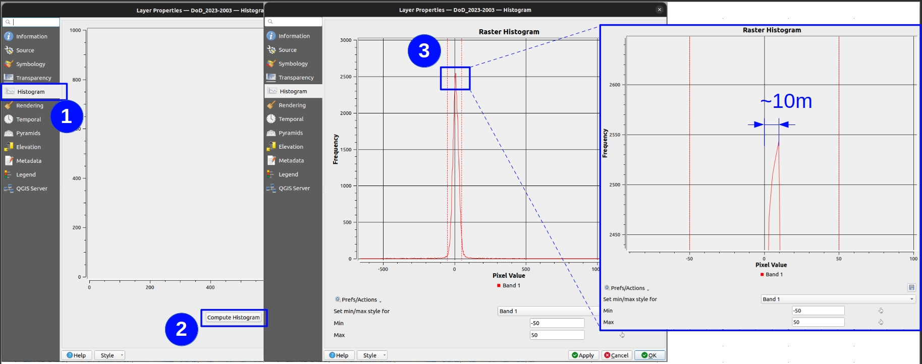
Fig. 5.3
Histogram of the DoD values DoD_2023-2003.tif file.
5.4.1.2. Aspect and slope calculation
In order to be able to use the co-registration procedure, you need first to compute slope and aspect. To do so in QGIS, please go to the toolbar section and within GDAL tools, you will find Aspect and Slope functions respectively. Since you are using the 2023 DEM as reference, for that procedure you will use the DEM corresponding to the 2003. The results should look very similar to Fig. 5.4.
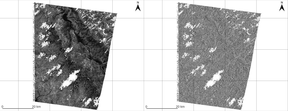
Fig. 5.4 Slope (left) and aspect (right) maps calculated from the 2003 DEM.
5.4.1.3. Random sampling of points
Once those results are generated, you will have to generate point samples from where coregistration will be calculated. To do so, you have to go to Vector -> Research Tools -> Random points in Extent. By using this tool Fig. 5.5, you will randomly generate 10 000 points shapefile based on the same extent of the Difference of DEM’s. The results of this procedure should look like in Fig. 5.6.
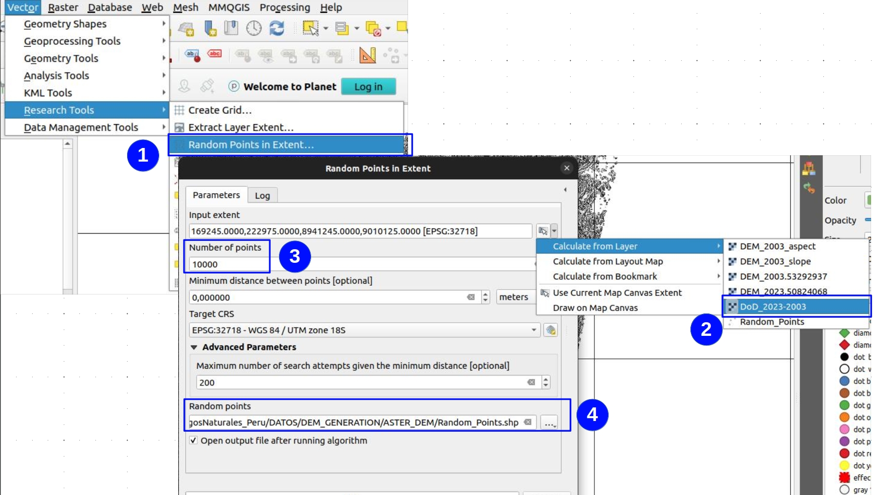
Fig. 5.5 Random points generation using QGIS.
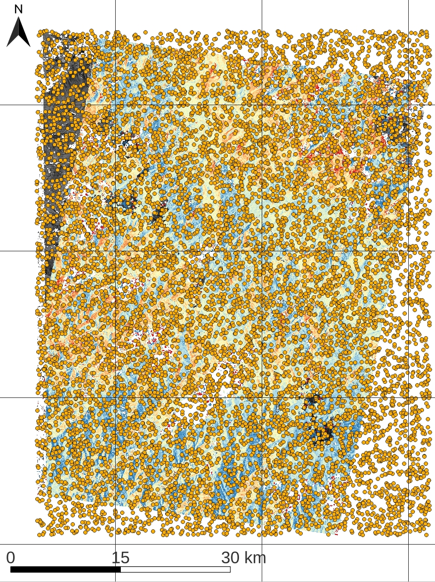
Fig. 5.6 Generated random points over the DoD raster.
5.4.1.4. Sampling the values of the rasters
Once the points are generated, you will have to extract the values of the DoD 2023-2003, slope and aspect rasters to the points. To do so, you will use the Point Sampling Tools plugin in QGIS. If you don’t have this plugin installed, please refer to the section Plugin -> Manage and Install Plugins, and type Point Sampling Tool. This plugin takes one point vector shapefile and several raster files to extract the value of the overlaid pixel, from the selected rasters. More information on the official webpage. You have to select the Random_points.shp file as well the raster files Fig. 5.7. Once the layers are selected, you can rename the columns to keep the column names clear and short Fig. 5.7. As a result, you will obtain a new shapefile that you will rename as Random_points_sample.shp but this time, you will find in the attribute table the columns you modified previously containing the pixel values from raster files Fig. 5.7.
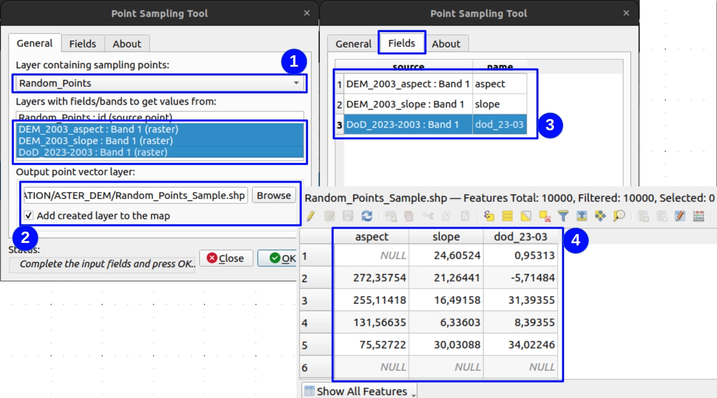
Fig. 5.7 Parameters on point sampling tool in QGIS.
5.4.1.5. Filtering point data with null values
As you may notice in the Fig. 5.6 and Fig. 5.7, there are several points which are located in empty areas, close to the image borders, for instance. These empty points or points containing missing (null) values, must be filtered/removed since they are not useful for the coregistration stage. To do so, you will open the attribute table of the Random_points_sample.shp and open the Select features using an expression tool. This option allows us to select the features by filling certain conditions (e.g., between a range of values, if values exist or not, etc). For this case, you will search those values with missing or null values inside the three columns (i.e., aspect, slope, dod_23-03). Inside Select features windows, you can have access to the columns by clicking in the Fields and Values option as well as the Operators that will be used to meet the searched conditions Fig. 5.8. Inside the box expression type the expression written in Fig. 5.8.
"aspect" is NULL OR "slope" is NULL OR "dod_23-03" is NULL
Note
aspect,slopeanddod_23-03= the fields or columns to be evaluated.is= in the operator/evaluator which compares each row of the columns selected previously.NULL= is the value of the expression to be fulfilled.OR= is the logical operator to allow us to select several columns and check if the condition is filled in one column in any column.
Questions for discussion
Why do we use the OR operator instead of AND?
By clicking on Select features, QGIS will select all features who meet the conditions for the three columns. The selection returns ~ 3830 points features. Since the point features were generated randomly, the selected points may differ for you. Finally, once you have selected the points, the final step is to delete them. To do so, you will Edit the points features and click on Delete selected. By doing so, we have reduced the initial point sample from 10 000 to 6 100 points. The results must look like Fig. 5.8.
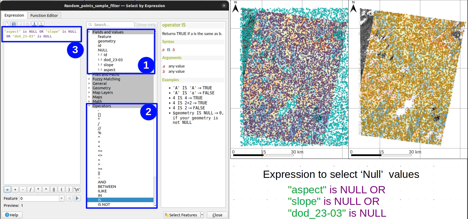
Fig. 5.8 Filtering points with null values using the expression tool in QGIS.
5.4.1.6. Filtering point with glacier outlines
Since the co-registration stage is based on those areas which have not suffered strong geomorphological changes (hereafter called as stable areas), you need to remove those points which are located within those areas which have strongly changed (i.e., glaciers, landslides, etc). So, you need to mask or remove those points within glacier outlines. To do so, you will use Randolph Glacier Inventory (RGI) version 7.0, as the main data source of glacier outlines. Please refer to the RGI documentation for more details about worldwide glacier inventory.
Once you have downloaded the shapefile of the glacier outlines, you will open it in QGIS and you will check that the coordinate reference system (CRS) is the same as your other layers. If not, you will have to reproject it to the same CRS (i.e. WGS84 UTM Zone 18S). Then, you will use the Select by location tool in QGIS to select those points within the glacier outlines Fig. 5.9. In this case, you will select features from Random_points_sample.shp that intersect with features from rgi60_SouthAmerica.shp. By clicking on Run, QGIS will select all points within the glacier outlines. Finally, you will delete those selected points by editing the layer and clicking on Delete selected. The final result should look like Fig. 5.9.
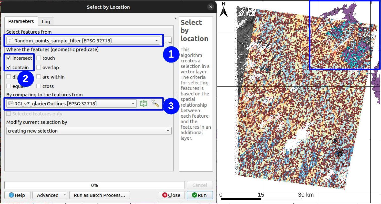
Fig. 5.9 Select points within glacier outlines using the Select by location tool in QGIS.
5.4.1.7. Exporting the point data to Excel
As a final step, you will export the attribute table of the remaining points. To do so, you will make right click on the layer Random_points_sample.shp and you will click on Save Features As…. Within the save vector layer menu you will change the format as MS Office Open XML spreadsheet [XLSX], which is the format excel. Finally, select the desired directory and click on OK; This procedure will export the entire attribute table in format excel.
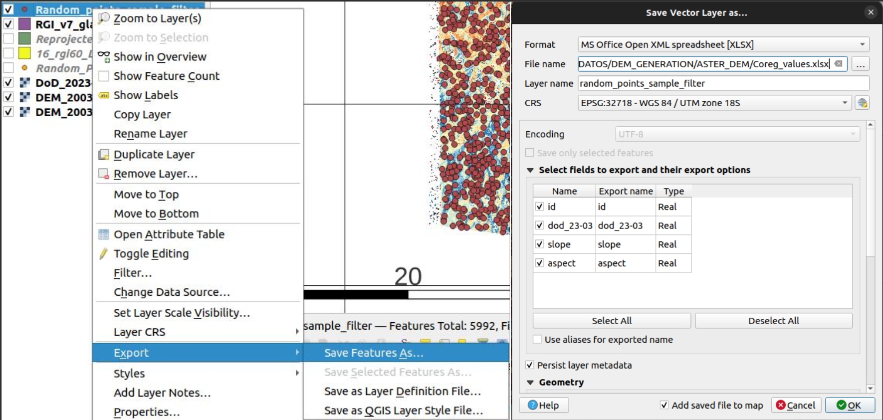
Fig. 5.10 Exporting point data to Excel from QGIS.
5.4.1.8. Co-registration in Excel
Make sure that Excel has
Solverinstalled. For general instructions on how load the Solver Add-in in Excel.Then open the
DEM Co-Registration Excel Toolprovided by Nuth and Kaab (2011). Can be downloaded here:Thirdly, open the random point sample excel file. Remember, for each record an elevation difference, and its corresponding slope and aspect values are mandatory. Copy the corresponding values and paste them in the columns A, B and C
INSERT RANDOM SAMPLE HERE. It might be necessary to adjust the formulas in columns D, E, F and RMSE in cell C6 to account for the size of the sample you have pasted.
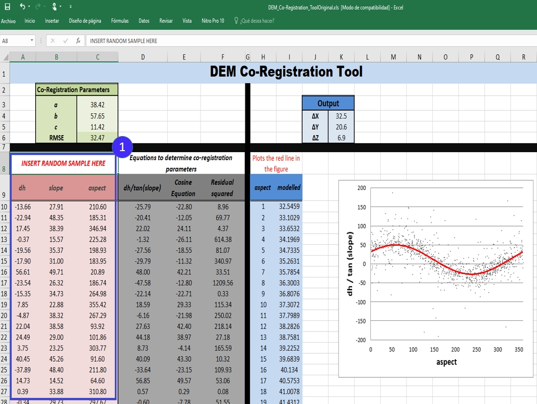
Fig. 5.11 DEM Co-Registration Excel Tool. The blue box shows the columns where the data input should be inserted.
Fourthly, use Solver to determine the co-registration parameters
ain cellC3,bin cellC4, andcin cellC5. To do so, set the parameters equal to 1 (initial value).
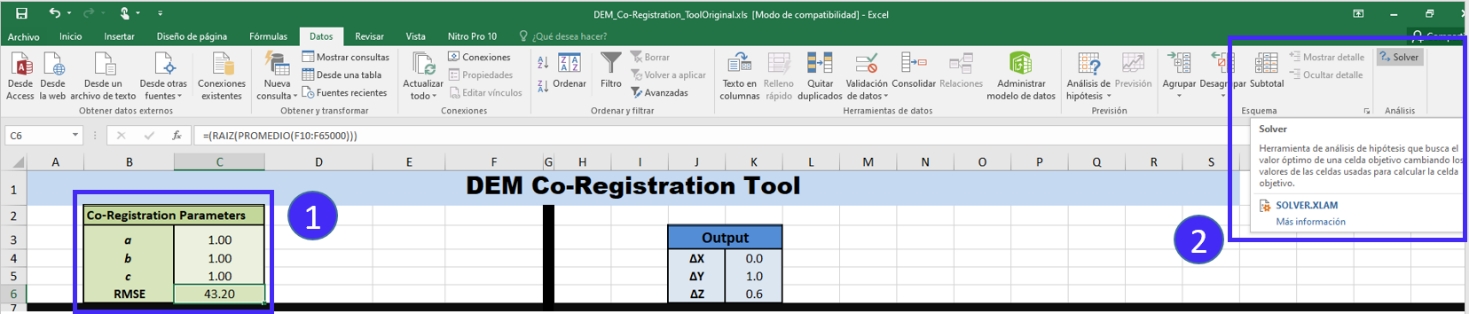
Fig. 5.12
Solver parameters to be set in the DEM Co-Registration Excel Tool.¶ Then, open solver configure the parameters as follows Fig. 5.13, Set Target Cell = C6, Equal to = Min, By Changing Cells C3:C5 and finally click on Solve.
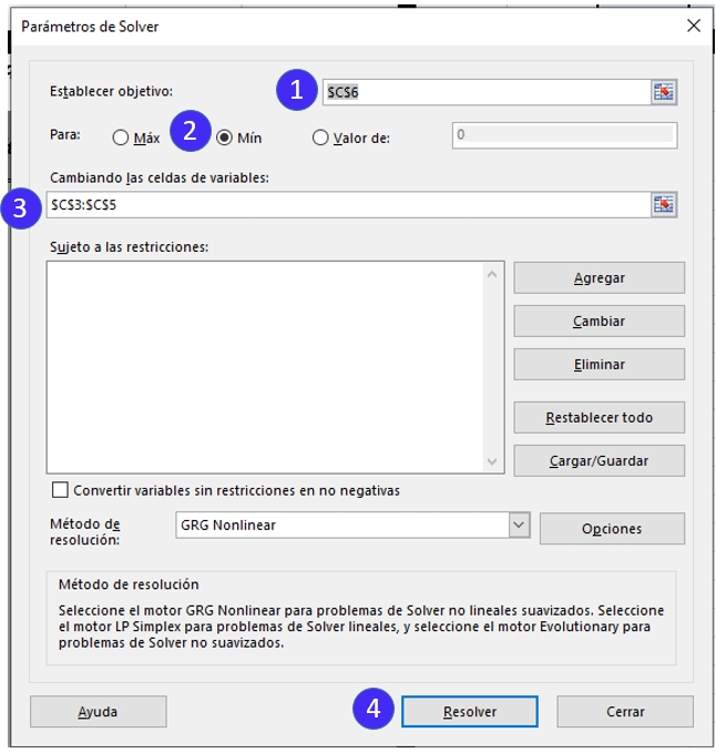
Fig. 5.13 Solver configuration to be set in the DEM Co-Registration Excel Tool.
The minimized solution is located in C3, C4, and C5. And the displacement values for geometrically adjustment are in K4, K5 and K6.
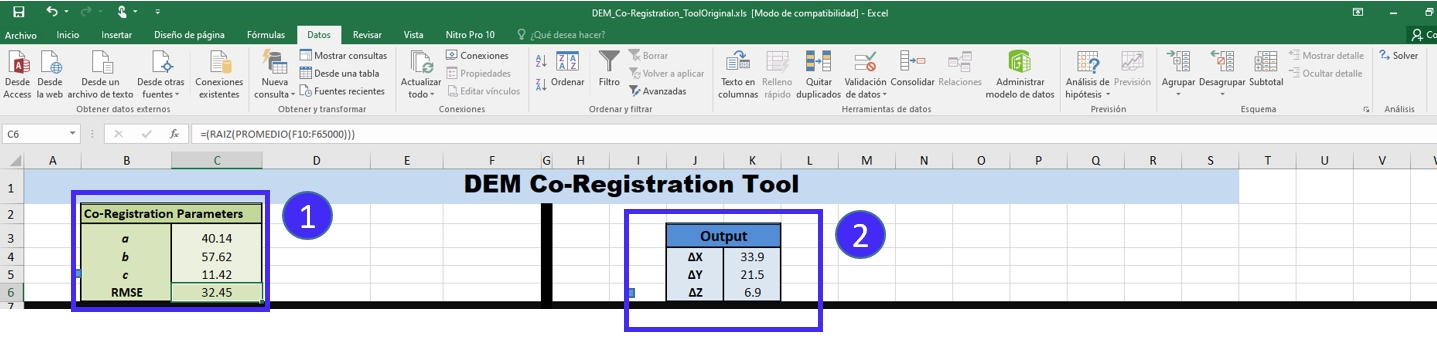
Fig. 5.14 Solver results in the DEM Co-Registration Excel Tool.
Finally, displacement x, y, z vector of correction is applied to the corner coordinates of the un-registered DEM. To this end you can use any QGIS through the translate tool. As we mention before, this is an iterative process, so repeat all the procedure until the red line fits through the points (Fig. 5.15). A good proxy to choose to stop the iteration is when the RMSE is improved up to 2% or if the magnitude of the displacement vector is less than 0.5 m.
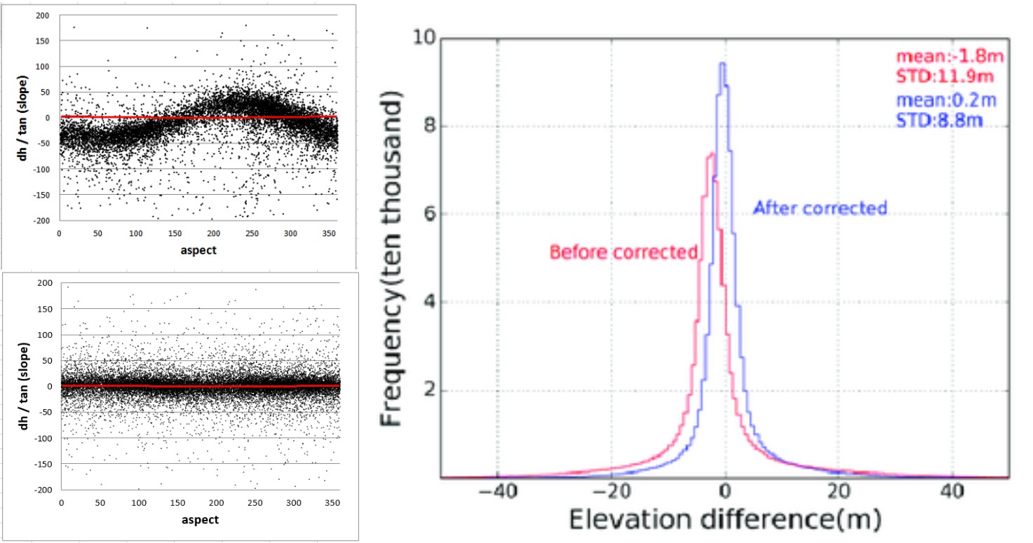
Fig. 5.15 Comparison of the elevation difference by the tangent of the slope, before and after coregistration, and the fitted cosine curve (red line). Example of the resulting histograms of the residuals after adjustment for bias.
Tip
Dem co-registration must be applied over stable rocky areas, so unstable areas should be removed.
The solution is most well defined for sample points on steeper slopes. Since
dh/tan(slope)cannot be defined flatted areas, zero slopes must be eliminated.A conic structure such as volcanos are perfect because it covers all terrain aspects as long as there is a sufficient amount of elevation difference samples.
Usually, less than 10000 samples are sufficient, although for the DEM Co-Registration excel tool it is possible to have up to 65000.
Using this tool, convergence is commonly obtained with less than ten iterations, depending the samples (number and distribution) and the fitting algorithm.
5.4.2. Automatic co-registration
In this second part of the exercise, you will learn how to apply the co-registration procedure in an automatic way using Python libraries. The main advantage of using this method is that it is not necessary to extract random points, filter them, export them to excel, etc. Everything is done in a single script.
Important
Download the data provided for this practice by running the following commands in your terminal:
Go to the /psf_telrisknat_2025_docs/data/ folder and run:
bash ./download_excercise_4_data.sh
5.4.2.1. Activation of the conda environment
First of all, you will activate the conda environment that you created in the practice Automatic generation of Digital Elevation Models using ASTER images. To do so, open a terminal and type:
conda activate psf_env
5.4.2.2. Get familiar with Geoutils library
Before starting with the co-registration procedure, you will get familiar with the Geoutils library. To do so, you will open a jupyter notebook by typing in the terminal:
jupyter notebook
Note
If you have some problems to open the jupyter notebook or is not installed, just run in your terminal:
mamba install -c conda-forge jupyter
This command will open a new tab in your web browser. Open the scrip called geoutils_introduction.ipynb provided in the data folder. This script will help you to understand how to use the main functions of the Geoutils library. Please, follow all the steps of the script.
5.4.2.3. Co-registration procedure using xDEM
Now, you will learn how to apply the co-registration procedure using the xDEM library. For this practice, you will use the same DEMs generated in the practice Automatic generation of Digital Elevation Models using ASTER images. The entire procedure is explained in the jupyter notebook called dem_coregistration.ipynb provided in the data folder.
5.4.2.4. Importing libraries and loading data
First, you should import the necessary libraries.
import matplotlib.pyplot as plt
import numpy as np

import geoutils as gu
import xdem

# To avoid interpolation in plt.imshow
plt.rcParams['image.interpolation'] = 'none'
Then, you will load the DEMs at once, croppping them to the same and reprojecting them to the same CRS.
fn_dem_2003 = "DEM_20030713.tif"
fn_dem_2023 = "DEM_20230704.tif"
fn_ref_dem = "COPDEM_30m.tif"
dem_2003, dem_2023, ref_dem = gu.raster.load_multiple_rasters([fn_dem_2003, fn_dem_2023, fn_ref_dem], crop=True, ref_grid=1)
ref_dem.set_nodata(-9999)
You can use the following code to visualize the DEMs.
fig, axs = plt.subplots(1, 3, figsize=(12, 6))
dem_2003.plot(ax=axs[0], cmap='terrain', title="DEM 2003")
dem_2023.plot(ax=axs[1], cmap='terrain', title="DEM 2023")
ref_dem.plot(ax=axs[2], cmap='terrain', title="Reference DEM")
plt.show()
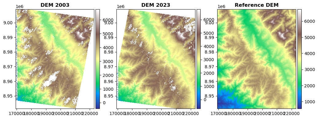
Fig. 5.16 Comparison of the three DEMs showing elevation data.
Then, you will also load and plot the glacier outlines.
rgi_shpfile = "Glaciares_Peru.shp"
rgi_outlines = gu.Vector(rgi_shpfile)
You may note that the Glaciares_Peru.shp layer contains nation-wide glacier inventory. However, glacier inventory uses different projection systems (e.g. WGS84). To solve this, you have to reproject the shapefile. In addition, we are working in the Cordillera Blanca region. So, you have to crop the shapefile to be compatible with the raster extent.
rgi_outlines.reproject(ref=dem_2023, inplace=True)
rgi_outlines_crop = rgi_outlines.crop(dem_2023)
rgi_outlines_crop.plot(color='blue', linewidth=1)
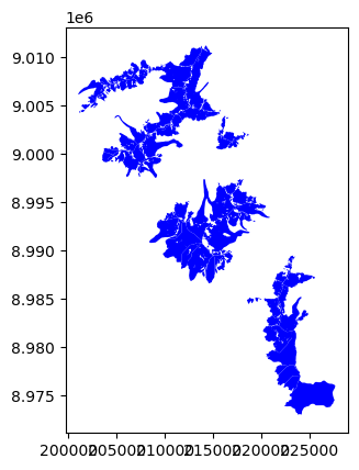
Fig. 5.17 Glacier outlines of the Cordillera Blanca region.
5.4.2.5. Computting the difference of DEMs (DoD)
Now, you will calculate the difference of DEMs (DoD) between the two DEMs and plot it.
dh2023 = dem_2023 - ref_dem
vmax=30
plt.figure(figsize=(6, 6))
ax = plt.subplot(111)
rgi_outlines.plot(ax=ax, facecolor='none', edgecolor='k', lw=0.5, zorder=2)
dh.plot(ax=ax, cmap='RdYlBu', vmin=-vmax, vmax=vmax, cbar_title='Elevation change 2012 - 2018 (m)', zorder=1)
ax.set_title('Cordillera Blanca and surroundings')
plt.tight_layout()
plt.show()
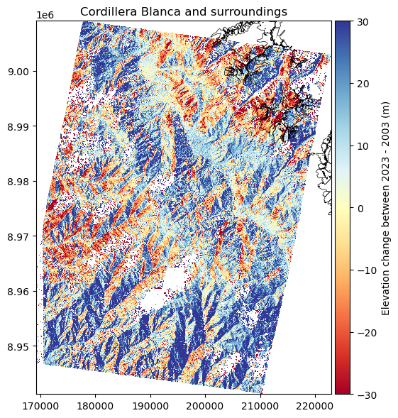
Fig. 5.18 Difference of DEMs (DoD) between 2023 and 2003.
5.4.2.6. Generating stable areas mask
Now, you have to select stable areas to compute the co-registration parameters. The selection os stable areas is done by masking everything that is not stable, i.e., glaciers and steep slopes. Regarding glacier mask, you can use the glacier outlines loaded previously to mask all glaciers.
gl_mask = rgi_outlines_crop.create_mask(dh)
Regarding slopes, you will use the reference DEM (COPDEM_30m.tif) to compute the slopes as it does not contain large voids. In this case, you will mask all slopes larger than 40 degrees.
slope = xdem.terrain.slope(ref_dem)
slope_mask = (slope.data < 40).filled(False)
outlier_mask = (np.abs(dh.data) < 50).filled(False)
Finally, you will combine all masks to get the stable areas.
inlier_mask = ~gl_mask.data.filled(False) & slope_mask & outlier_mask
plt.figure(figsize=(8, 8))
plt.imshow(inlier_mask.squeeze()) # squeeze to remove the singleton dimension??
plt.show()
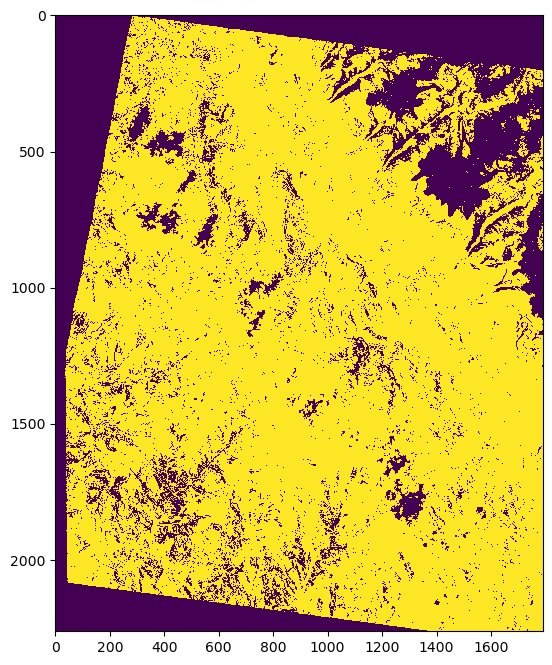
Fig. 5.19 Stable areas (True values) used for the co-registration procedure.
5.4.2.7. Applying the co-registration
Now, you are ready to apply the co-registration procedure. For this excercise, you will use Nuth and Kaab (2011):cite:nuth2011 method implemented in the xDEM library. First, we need to define the coregistration function. Then we estimate the coregistration needed between our two ASTER DEMs. Finally, we apply that coregistration to the 2003 DEM.
coreg = xdem.coreg.NuthKaab() + xdem.coreg.VerticalShift(vshift_reduc_func=np.median)
coreg.fit(dem_2023, dem_2003, inlier_mask, verbose=True)
dem_2003_coreg = coreg.apply(dem_2003)
You can visualize the results of the co-registration procedure by inspecting metadata of the coreg object.
print(coreg.pipeline[0]._meta)
Questions for discussion
What are the estimated shifts in x, y and z?
How many iterations were needed to converge?
Now, you can compute the DoD between the co-registered 2003 DEM and the 2023 DEM and plot it.
dh_coreg = dem_2023 - dem_2003_coreg
vmax = 50
fig, (ax1, ax2, ax3) = plt.subplots(1, 3, figsize=(15, 6))
rgi_outlines_crop.plot(ax=ax1, facecolor='none', edgecolor='k', zorder=3)
dh.plot(ax=ax1, cmap='RdYlBu', vmin=-vmax, vmax=vmax, cbar_title='Elevation change 2012 - 2018 (m)', zorder=1)
ax1.set_title('Before coregistration')

rgi_outlines_crop.plot(ax=ax2, facecolor='none', edgecolor='k', zorder=3)
dh_coreg.plot(ax=ax2, cmap='RdYlBu', vmin=-vmax, vmax=vmax, cbar_title='Elevation change 2012 - 2018 (m)', zorder=1)
ax2.set_title('After coregistration')

ax3.set_title('Elevation change distribution')
ax3.hist(dh.data.compressed(), bins=100, alpha=0.5, label='Before', range=(-vmax, vmax), color='blue')
ax3.hist(dh_coreg.data.compressed(), bins=100, alpha=0.5, label='After', range=(-vmax, vmax), color='green')
ax3.set_xlabel('Elevation change (m)')
ax3.set_ylabel('Frequency')
ax3.legend()

plt.tight_layout()
plt.show()
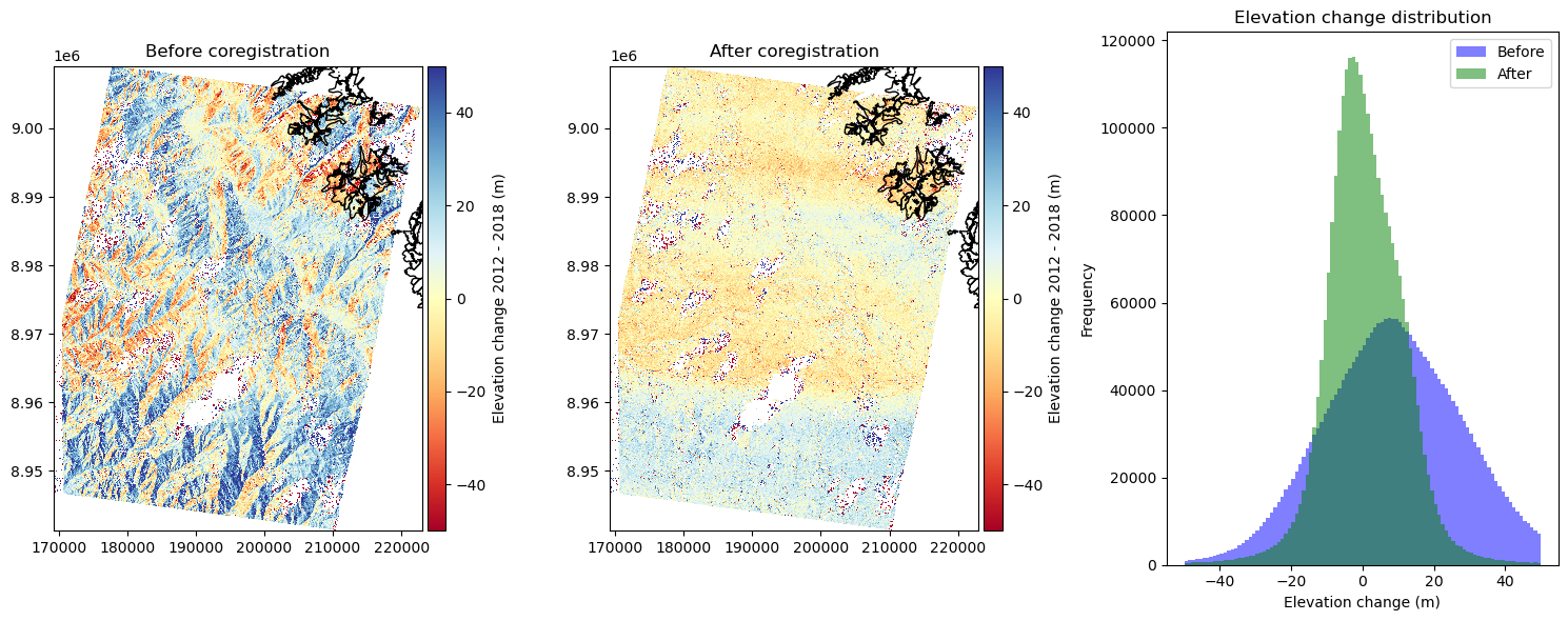
Fig. 5.20 Comparison of the DoD before (left) and after (middle) co-registration, and the histograms of the DoD values (right).
Questions for discussion
How has the DoD changed after co-registration?
How has the distribution of DoD values changed after co-registration?
5.4.2.8. Computting statistics on stable areas
You can also compute some statistics on the stable areas before and after co-registration.
inlier_orig = dh[inlier_mask]
nstable_orig, mean_orig = len(inlier_orig), np.mean(inlier_orig)
med_orig, nmad_orig = np.median(inlier_orig), xdem.spatialstats.nmad(inlier_orig)
print(f"Number of stable pixels: {nstable_orig}")
print(f"Before coregistration:\
      \n\tMean dh: {mean_orig:.2f}\
      \n\tMedian dh: {med_orig:.2f}\
      \n\tNMAD dh: {nmad_orig:.2f}")

inlier_coreg = dh_coreg[inlier_mask]
nstable_coreg, mean_coreg = len(inlier_coreg), np.mean(inlier_coreg)
med_coreg, nmad_coreg = np.median(inlier_coreg), xdem.spatialstats.nmad(inlier_coreg)
print(f"After coregistration:\
      \n\tMean dh: {mean_coreg:.2f}\
      \n\tMedian dh: {med_coreg:.2f}\
      \n\tNMAD dh: {nmad_coreg:.2f}")
5.4.2.9. Saving the results
Finally, you can save the co-registered DEM.
dem_2003_coreg.save("DEM_20230704_coreg.tif")
dh_coreg.save("DoD_20230704_20030713_coreg.tif")
5.5. References
Joan A. Casey, Yuqian M. Gu, Lara Schwarz, Timothy B. Frankland, Lauren B. Wilner, Heather McBrien, Nina M. Flores, Arnab K. Dey, Gina S. Lee, Chen Chen, Tarik Benmarhnia, and Sara Y. Tartof. The 2025 Los Angeles Wildfires and Outpatient Acute Healthcare Utilization. medRxiv, pages 2025.03.13.25323617, March 2025. doi:10.1101/2025.03.13.25323617.
Jon E. Keeley and Alexandra D. Syphard. Large California wildfires: 2020 fires in historical context. Fire Ecology, 17(1):22, August 2021. doi:10.1186/s42408-021-00110-7.
Pascal Lacroix, Gael Araujo, James Hollingsworth, and Edu Taipe. Self-Entrainment Motion of a Slow-Moving Landslide Inferred From Landsat-8 Time Series. Journal of Geophysical Research: Earth Surface, 124(5):1201–1216, 2019. _eprint: https://agupubs.onlinelibrary.wiley.com/doi/pdf/10.1029/2018JF004920. URL: https://onlinelibrary.wiley.com/doi/abs/10.1029/2018JF004920 (visited on 2023-03-01), doi:10.1029/2018JF004920.
Laura Parra García, Gianluca Furano, Max Ghiglione, Valentina Zancan, Ernesto Imbembo, Christos Ilioudis, Carmine Clemente, and Paolo Trucco. Advancements in Onboard Processing of Synthetic Aperture Radar (SAR) Data: Enhancing Efficiency and Real-Time Capabilities. IEEE Journal of Selected Topics in Applied Earth Observations and Remote Sensing, 17:16625–16645, 2024. doi:10.1109/JSTARS.2024.3406155.
Diego Cusicanqui, Antoine Rabatel, Christian Vincent, Xavier Bodin, Emmanuel Thibert, and Bernard Francou. Interpretation of Volume and Flux Changes of the Laurichard Rock Glacier Between 1952 and 2019, French Alps. Journal of Geophysical Research: Earth Surface, 126(9):e2021JF006161, October 2021. doi:10.1029/2021JF006161.
Yifei Zhu, Xin Yao, Leihua Yao, and Chuangchuang Yao. Detection and characterization of active landslides with multisource SAR data and remote sensing in western Guizhou, China. Natural Hazards, 111(1):973–994, March 2022. doi:10.1007/s11069-021-05087-9.
Pascal Lacroix, Amaury Dehecq, and Edu Taipe. Irrigation-triggered landslides in a Peruvian desert caused by modern intensive farming. Nature Geoscience, 13(1):56–60, January 2020. Number: 1 Publisher: Nature Publishing Group. URL: https://www.nature.com/articles/s41561-019-0500-x (visited on 2023-03-01), doi:10.1038/s41561-019-0500-x.
David P. Roy, Haiyan Huang, Rasmus Houborg, and Vitor S. Martins. A global analysis of the temporal availability of PlanetScope high spatial resolution multi-spectral imagery. Remote Sensing of Environment, 264:112586, October 2021. doi:10.1016/j.rse.2021.112586.
Swann Zerathe, Pascal Lacroix, Denis Jongmans, Jersy Marino, Edu Taipe, Marc Wathelet, Walter Pari, Lionel Fidel Smoll, Edmundo Norabuena, Bertrand Guillier, and Lucile Tatard. Morphology, structure and kinematics of a rainfall controlled slow-moving Andean landslide, Peru. Earth Surface Processes and Landforms, 41(11):1477–1493, 2016. doi:10.1002/esp.3913.
Noélie Bontemps, Pascal Lacroix, and Marie-Pierre Doin. Inversion of deformation fields time-series from optical images, and application to the long term kinematics of slow-moving landslides in Peru. Remote Sensing of Environment, 210:144–158, June 2018. doi:10.1016/j.rse.2018.02.023.
Francois Ayoub, Sebastien Leprince, Renaud Binet, Kevin W. Lewis, Oded Aharonson, and Jean Philippe Avouac. Influence of camera distortions on satellite image registration and change detection applications: 2008 IEEE International Geoscience and Remote Sensing Symposium - Proceedings. 2008 IEEE International Geoscience and Remote Sensing Symposium - Proceedings, pages II1072–II1075, December 2008. doi:10.1109/IGARSS.2008.4779184.
Theodore A. Scambos, Melanie J. Dutkiewicz, Jeremy C. Wilson, and Robert A. Bindschadler. Application of image cross-correlation to the measurement of glacier velocity using satellite image data. Remote Sensing of Environment, 42(3):177–186, December 1992. doi:10.1016/0034-4257(92)90101-O.
Ross A. Beyer, Oleg Alexandrov, and Scott McMichael. The ames stereo pipeline: nasa's open source software for deriving and processing terrain data. Earth and Space Science, 5(9):537–548, 2018. doi:10.1029/2018EA000409.
David E. Shean, Oleg Alexandrov, Zachary M. Moratto, Benjamin E. Smith, Ian R. Joughin, Claire Porter, and Paul Morin. An automated, open-source pipeline for mass production of digital elevation models (dems) from very-high-resolution commercial stereo satellite imagery. ISPRS Journal of Photogrammetry and Remote Sensing, 116:101–117, 2016. doi:10.1016/j.isprsjprs.2016.03.012.
Diego Cusicanqui, Pascal Lacroix, Xavier Bodin, Benjamin Aubrey Robson, Andreas Kääb, and Shelley MacDonell. Detection and reconstruction of rock glacier kinematics over 24 years (2000–2024) from Landsat imagery. The Cryosphere, 19(7):2559–2581, July 2025. doi:10.5194/tc-19-2559-2025.
Martin Mergili, Adam Emmer, Anna Juřicová, Alejo Cochachin, Jan-Thomas Fischer, Christian Huggel, and Shiva P. Pudasaini. How well can we simulate complex hydro-geomorphic process chains? The 2012 multi-lake outburst flood in the Santa Cruz Valley (Cordillera Blanca, Perú). Earth Surface Processes and Landforms, 43(7):1373–1389, 2018. doi:10.1002/esp.4318.
I. Dussaillant, E. Berthier, F. Brun, M. Masiokas, R. Hugonnet, V. Favier, A. Rabatel, P. Pitte, and L. Ruiz. Two decades of glacier mass loss along the andes. Nature Geoscience, 12(10):802–808, 2019. doi:10.1038/s41561-019-0432-5.
D. Schneider, C. Huggel, A. Cochachin, S. Guillén, and J. García. Mapping hazards from glacier lake outburst floods based on modelling of process cascades at lake 513, carhuaz, peru. In Advances in Geosciences, volume 35, 145–155. 2014. URL: https://adgeo.copernicus.org/articles/35/145/2014/, doi:10.5194/adgeo-35-145-2014.
Diego Cusicanqui and Xavier Bodin. Photogrammetry for the study of mountain slopes. Webinar at INDURA, 2019. URL: https://vimeo.com/473376992.
Hideyuki Tonooka and Tetsushi Tachikawa. Aster cloud coverage assessment and mission operations analysis using terra/modis cloud mask products. Remote Sensing, 11(23):2798, 2019. doi:10.3390/rs11232798.
INAIGEM. Inventario nacional de glaciares y lagunas de origen glaciar 2023. Technical Report, Instituto Nacional de Investigación en Glaciares y Ecosistemas de Montaña, 2023. URL: https://hdl.handle.net/20.500.12748/499.
Romain Hugonnet, Robert McNabb, Etienne Berthier, Brian Menounos, Christopher Nuth, Luc Girod, Daniel Farinotti, Matthias Huss, Ines Dussaillant, Fanny Brun, and Andreas Kääb. Accelerated global glacier mass loss in the early twenty-first century. Nature, 592(7856):726–731, 2021. doi:10.1038/s41586-021-03436-z.
Fanny Brun, Etienne Berthier, Patrick Wagnon, Andreas Kääb, and Désirée Treichler. A spatially resolved estimate of high mountain asia glacier mass balances from 2000 to 2016. Nature Geoscience, 10(9):668–673, 2017. doi:10.1038/ngeo2999.
C. Nuth and A. Kääb. Co-registration and bias corrections of satellite elevation data sets for quantifying glacier thickness change. The Cryosphere, 5(1):271–290, March 2011. doi:10.5194/tc-5-271-2011.
A. Federico, M. Popescu, G. Elia, C. Fidelibus, G. Internò, and A. Murianni. Prediction of time to slope failure: a general framework. Environmental Earth Sciences, 66(1):245–256, May 2012. doi:10.1007/s12665-011-1231-5.
Mathilde Desrues, Pascal Lacroix, and Ombeline Brenguier. Satellite Pre-Failure Detection and In Situ Monitoring of the Landslide of the Tunnel du Chambon, French Alps. Geosciences, 9(7):313, July 2019. doi:10.3390/geosciences9070313.
Teruki Fukuzono. A new method for predicting the failure time of slope. In Proceedings, 4th Int'l. Conference and Field Workshop on Landslides, 145–150. 1985.
M Saito. Forecasting time of slope failure by tertiary creep. In Proceedings of 7th International Conference on Soil Mechanics and Foundation Engineering, 1969, volume 2, 677–683. 1969.
A. Segalini, A. Valletta, and A. Carri. Landslide time-of-failure forecast and alert threshold assessment: A generalized criterion. Engineering Geology, 245:72–80, November 2018. doi:10.1016/j.enggeo.2018.08.003.