2. Change detection using optical images
Floriane PROVOST1, Pascal LACROIX2 & Diego CUSICANQUI2
1 Institut de Physique du Globe de Strasbourg, EOST/Université de Strasbourg, Strasbourg, France
2 Univ. Grenoble Alpes, CNES, CNRS, IRD, Institut des Sciences de la Terre (ISTerre), Grenoble, France.
Copyright
Document version 0.2, Last update: 2025-09-18
© PSF TelRIskNat 2025 Optical team (D. Cusicanqui, R. Basantes & P. Lacroix). This document and its contents are licensed under the Creative Commons Attribution 4.0 International License (CC BY-NC-SA 4.0).
2.1. Learning objectives:
Design a workflow to answer a question
Learn how to create RGB composite and to compute indexes
Learn how to create manually a vector file
Execute spatial/attribute operations to create a vector file
Create a map that summarise your results
2.2. Introduction
We are going to study the wild fires that impacted California in January 2025. The main goal of our study is to estimate how many houses/building were destroyed by the 2025 wild fire?
Regarding the California wild fire event, In 2024, the San Francisco Bay Area experienced several notable wildfires around the region rather than inside the city itself. The Corral Fire near Tracy in the Diablo Range burned about 14,168 acres (≈ 57.34 km²) from June 1–6, while Sonoma County’s Point Fire scorched ~1,207 acres (≈ 4.88 km²) from June 16–24. More infor in CallFire.
Smoke from these and other regional fires periodically drifted into San Francisco, prompting Bay Area Air Quality Management District advisories—especially in mid-June and again in August—due to hazy skies and particle pollution concerns [1]. Overall, impacts in San Francisco were felt mainly through smoke and reduced air quality, while the largest burn areas were in surrounding counties SFGATE. More information about large California wildfires in [2]
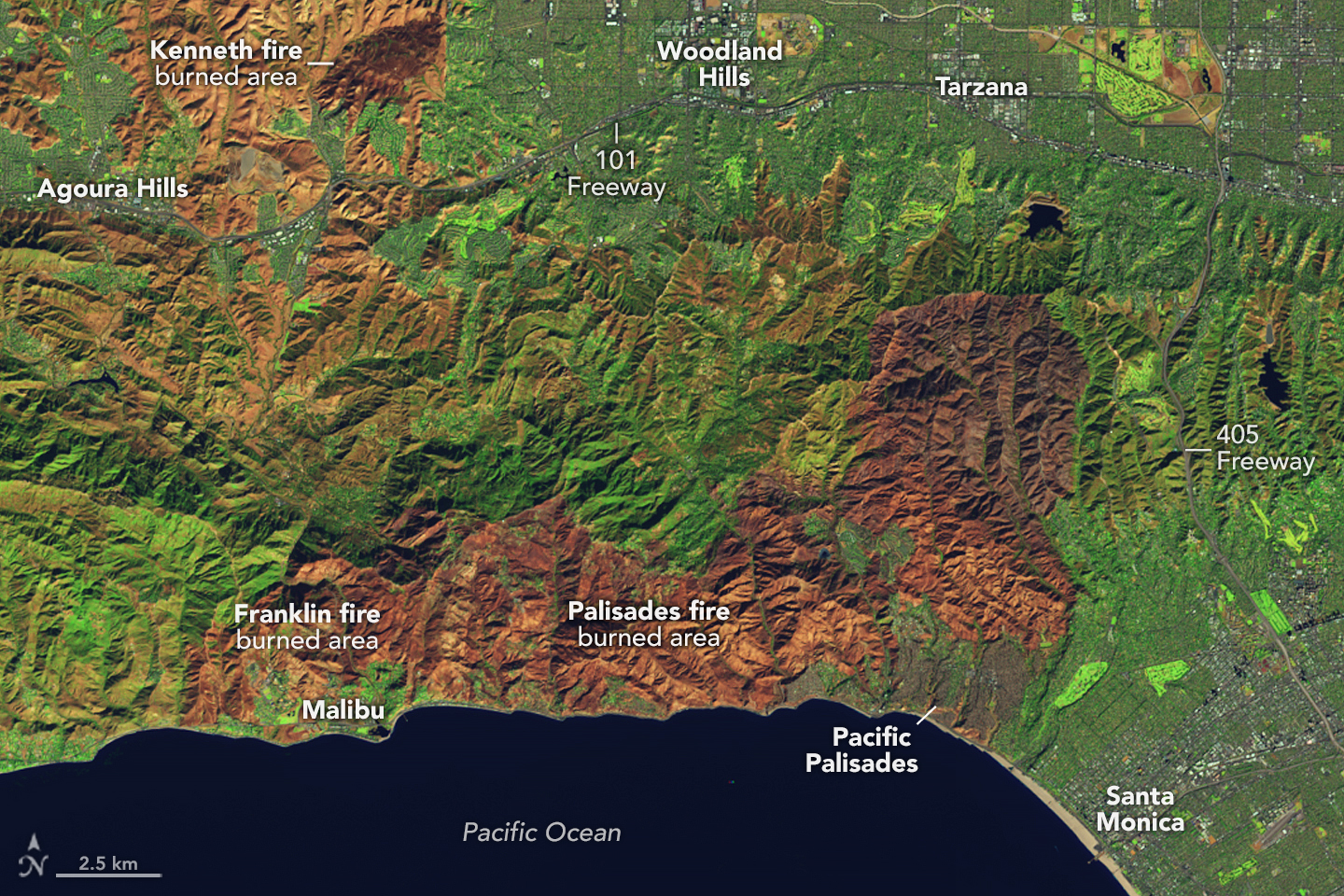
Fig. 2.1 Wildfire in California, USA. Source: NASA Earth Observatory.
First of all, try to draft a workflow/diagram describing the logical steps and operations needed to answer the question. For that, answer to these questions:
What data do you need?
What information do you need?
What operation do you need to execute to obtain the results?
Once answered construct the diagram.
2.3. Raster data
We need to map the wild fire extent. To do that we are going to use Sentinel-2 images and manipulate the bands in order to easily detect and map the fires.
For this practice, we are going to use QGIS independent of the operating system. If you have not installed QGIS yet, please refer to the practical Installation.
Tip
Download the data using the following link RENATER (valid until 2025-12-31).
2.3.1. Sentinel-2 images
The Sentinel-2 images are available on the Copernicus Open Access Hub or AWS. For this practical, we provide you two Sentinel-2 images acquired before and after the fire event. The data is located in the two separate folders in data/exercise_1_change_detection named by their acquisition date.
S2_L1C_T11SLT_20250102T183751(before the fire event)S2_L1C_T11SLT_20250112T183731(after the fire event)
Note
Load all the bands on QGIS and compare them. Do you see the wild fires?
2.3.2. Sentinel-2 RGB composite
Sentinel-2 images are multispectral images, meaning that they contain several bands acquired at different wavelengths. Visit: Sentinel Hub to determine what RGB is more suitable to map wildfires.
Now, create a RGB composite for both dates (before and after the fire event).
- Open the menu Raster > Miscellaneous > Create a Virtual Raster…
- Define the bands composing the RGB composite.
- Click on Place each input file into a separate band.
- Create the Virtual raster.
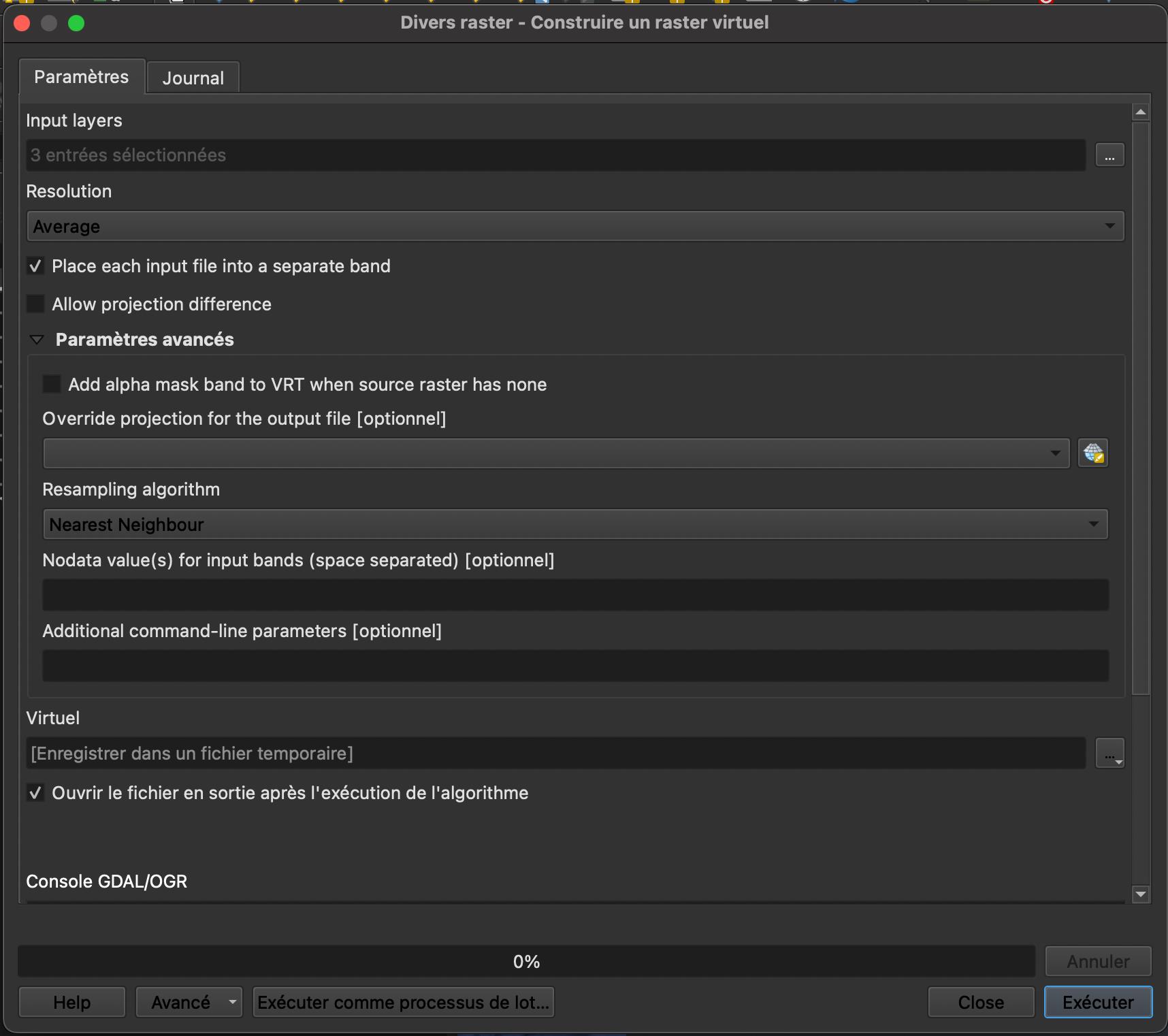
Fig. 2.2 Sentinel-2 RGB composite.
2.3.3. Sentinel-2 band math
As fires are burning the vegetation, another option is to compute the Normalised Different Vegetation index (NDVI). This index is a widely used metric for quantifying the health and density of vegetation. Compute the NDVI by opening the function Raster > Raster Calculator. This window should appear as Fig. 2.3.
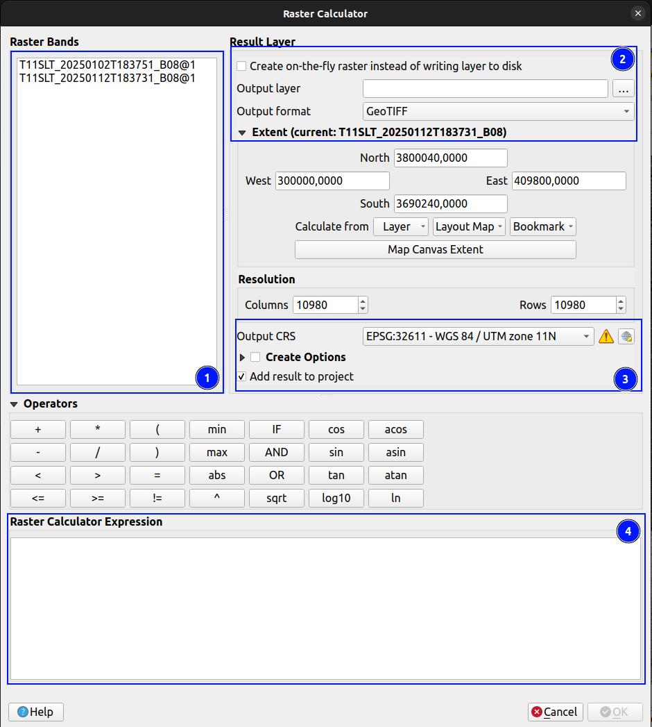
Fig. 2.3 Sentinel-2 NDVI.
Define the mathematical operation you want to realize (here NDVI). Be careful, select bands of the same date.
Choose to
create the raster "on-the-fly"or to save it in your project (preferred). If you choose to create the raster on-the-fly, the raster will appear in the project but will not be saved. If you save the project, close it and open it later, the raster will be empty (because it was not saved).Repeat the operation for the two dates of acquisition.
Important
It’s important that your data are well organised ! Both in your computer and in QGIS. For example, layers can be grouped together to organise the layer browser in QGIS.
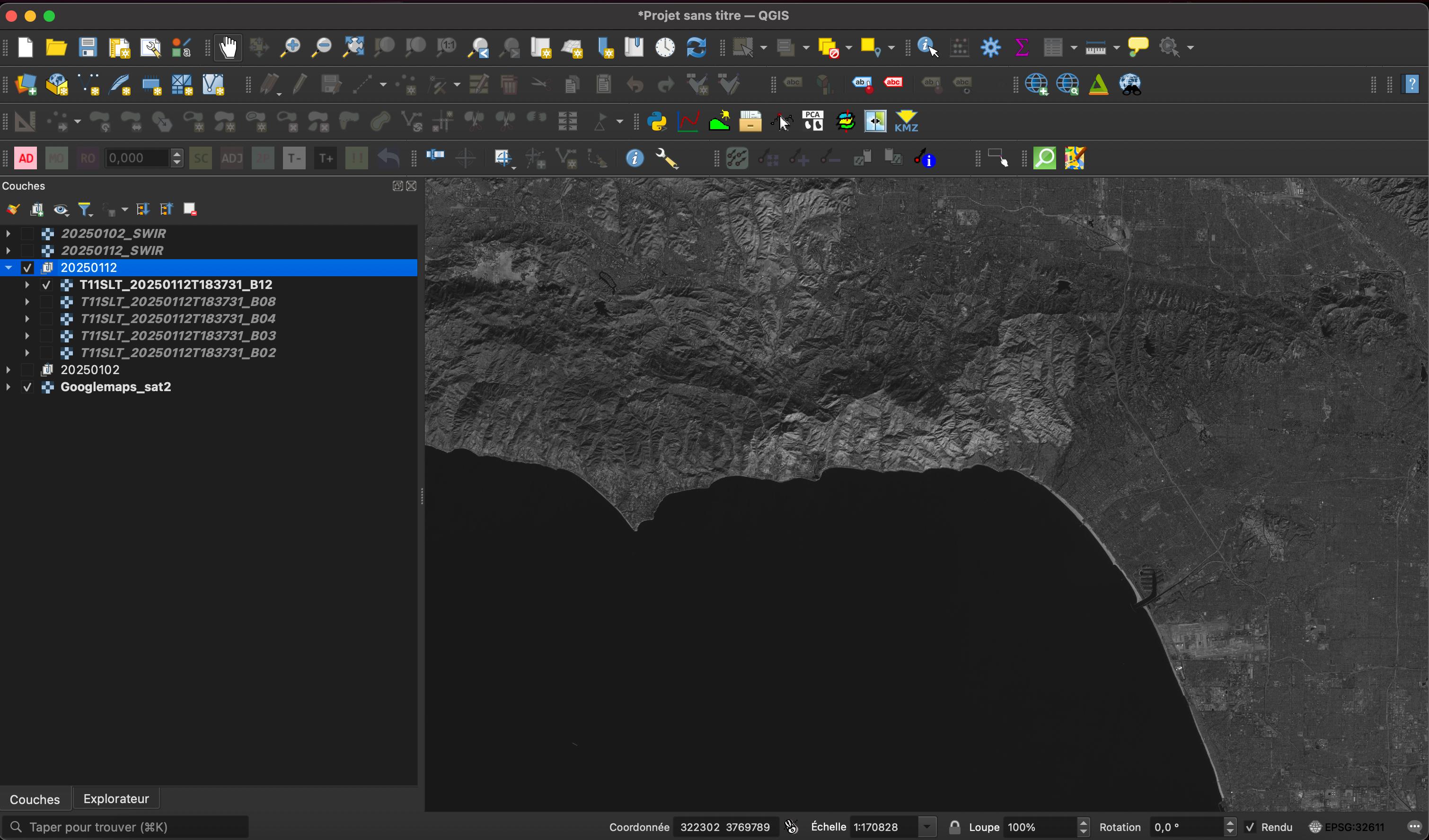
Fig. 2.4 Sentinel-2 NDVI change.
2.4. Vector data
2.4.1. Manually create a vector file
Vector files can be created manually with the function XXX The following window should appear like Fig. 2.5.
Choose the name of the file, the extension (shapefile), and set up carefully the geometry (point, line or polygon) and the CRS. Click
OKonce all the options have been chosen. The layer should appear in the sectionLayersof the GIS environment.To edit the layer, click on the created vector file and on the function
Toggle Editing(pencil icon).Click then on the function
Add Polygon Feature(yellow star icon) to create a new entity.Click on the map to draw the limits of the polygon you want to map.
Save the entity by clicking on the function
Save Layer Edits(floppy disk icon) to render the layer non editable.If you want to modify the points/shape of your vector, use the function
Vertex Tool(icon with a point and a line) and move/modify the points.
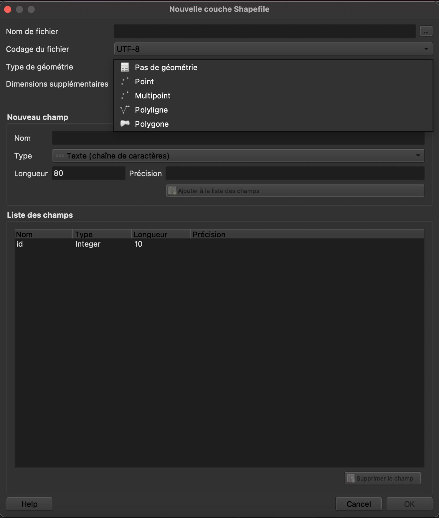
Fig. 2.5 Create a vector file manually.
Do it yourself
Map manually the fire extent(at least the eastern fire located north of Pasadena).
2.4.2. Create a vector file from raster data
Now, we are going to create a vector file from the NDVI change raster. The idea is to extract the area where the NDVI has decreased significantly (i.e. vegetation has been destroyed by the fire).
a. Determine what operation should be realized to extract the fire extent from the NDVI
raster files. Use the Raster Calculator to derive a raster with the fire extent.
Vectorize the resulting raster using the function
Raster > Conversion > Raster to Polygon. You should obtain a new vector layer that looks like Fig. 2.6. The spatial domain is correctly sampled into geographical entities but many geographical entities are not of interest for this study.
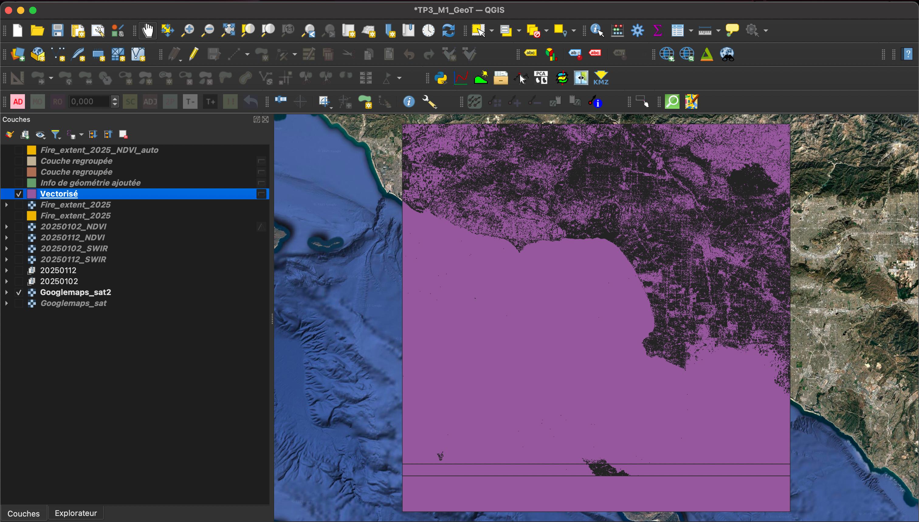
Fig. 2.6 Create a vector file from a raster.
Questions for discussion
What entities should be filtered?
What attribute/properties do we need to compute to it?
Use the function
Vector > Geometry > add geometrical attributesto compute the area and perimeter of each entity of the vector layerVectorized.Use the attribute table to filter entities with areas smaller than 1,000 m², remove them by editing the table
Toggle Editing(pencil icon) and deleting the selected entities (red garbage).Repeat the operation to remove entities with areas larger than 68,000,000 m².
Regroup the entities in one single entity
fire extentby using the functionVector > Geoprocessing Tools > Dissolve. Your final result should look like Fig. 2.7.
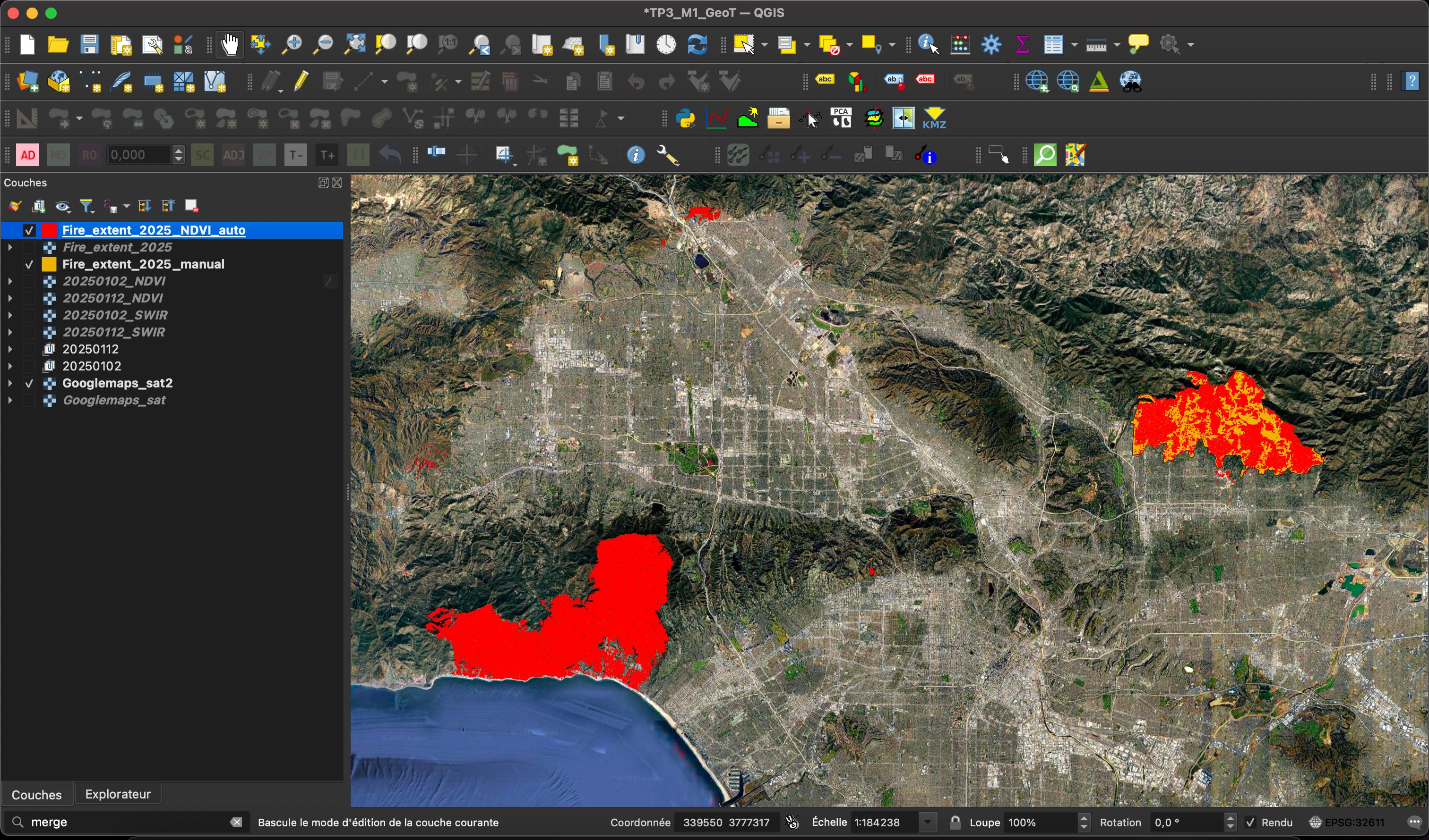
Fig. 2.7 Fire extent vector file.
Create a map showing the extent of the fires in California in January 2025.
2.5. Quantifying impacts
2.5.1. Count the number of buildings destroyed
To estimate the number of buildings destroyed by the fire, we are going to use a vector file containing the building footprints in California. The file is located in data/exercise_1_change_detection/buildings_CA.shp.
Load the vector file
buildings_CA.shpin QGIS.Use the function
Vector > Geoprocessing Tools > Intersectionto extract the buildings that intersect the fire extent.Open the attribute table of the resulting vector layer and count.
Questions for discussion
How many building were impacted?
Estimate the total surface of damaged building by performing an operation on the
Attribute table.Estimate the cost of the wildfire (price per square meter in California is ranging from 500$ to 700$).
2.5.2. Check our mapping
We are now going to use Open Street Map (OSM) to check our mapping. OSM data is a geographic database feed by a community of mappers that contribute and maintain data about roads, trails. It is therefore possible to download the raw data directly and reuse it as you wish, for cartographic or other purposes. Every week, a complete file called planet is generated and made available by the OpenStreetMap Foundation. This file is very large and growing fast (20 GB at the end of 2011, 63 GB at the beginning of 2018) because it contains all the data for the entire planet. Extracts by continent, country or region are also available and updated daily by Geofabrik. There are also tools for breaking down a file into smaller geographical areas.
There are several ways of viewing and downloading OSM data:
2.5.2.1. Viewing the ‘static’ OSM map
The ‘static’ OSM map represents OSM data in raster form. It is not possible to manipulate the information contained in this layer. However, it allows OSM information to be viewed and can be used as a background map. To download the OSM map into QGIS you need to use the QuickMapServices extension.
Display OSM from WMS layers already installed on your computer. Use the function Web > QuickMapServices > OSM > OSM Standard. Look at the areas affected by the fires. What do you notice?
2.5.2.2. Download the OSM database for an area of interest
You can download OSM data using QuickOSM plugin to download the vector data from the OSM base maps.
Click on the function
Vector > QuickOSM > QuickOSM(green lupe icon).Click on
Themeand select the defaultUrbantheme. Define the geographical extent for which you want to download the data. You can use theCanvas extentoption to download the data for the area currently displayed on your QGIS canvas.
Important
This area must not be too large, as this could create a memory problem in QGIS.
Click on
Execute queryto download the data. Several layers should appear in yourLayerssection.
You can also use the OSMDownloader plugin to download OSM data. This plugin allows you to download OSM data in a specific format (shapefile, geopackage, etc.) and for a specific area of interest.
Install the plugin OSMDownloader from the QGIS plugin manager.
Open the plugin from the menu
OSMDownloader.Define the area of interest by drawing a rectangle.
Save the data in a specific format (shapefile, geopackage, etc.) and download.
A number of vector layers should appear in your Layers tab. Manipulate these layers to
display the buildings mapped in OSM and compare with your result.
Do it yourself
Draw a diagram that represents all the steps realised to answer the initial question.
2.6. References
Joan A. Casey, Yuqian M. Gu, Lara Schwarz, Timothy B. Frankland, Lauren B. Wilner, Heather McBrien, Nina M. Flores, Arnab K. Dey, Gina S. Lee, Chen Chen, Tarik Benmarhnia, and Sara Y. Tartof. The 2025 Los Angeles Wildfires and Outpatient Acute Healthcare Utilization. medRxiv, pages 2025.03.13.25323617, March 2025. doi:10.1101/2025.03.13.25323617.
Jon E. Keeley and Alexandra D. Syphard. Large California wildfires: 2020 fires in historical context. Fire Ecology, 17(1):22, August 2021. doi:10.1186/s42408-021-00110-7.
Pascal Lacroix, Gael Araujo, James Hollingsworth, and Edu Taipe. Self-Entrainment Motion of a Slow-Moving Landslide Inferred From Landsat-8 Time Series. Journal of Geophysical Research: Earth Surface, 124(5):1201–1216, 2019. _eprint: https://agupubs.onlinelibrary.wiley.com/doi/pdf/10.1029/2018JF004920. URL: https://onlinelibrary.wiley.com/doi/abs/10.1029/2018JF004920 (visited on 2023-03-01), doi:10.1029/2018JF004920.
Laura Parra García, Gianluca Furano, Max Ghiglione, Valentina Zancan, Ernesto Imbembo, Christos Ilioudis, Carmine Clemente, and Paolo Trucco. Advancements in Onboard Processing of Synthetic Aperture Radar (SAR) Data: Enhancing Efficiency and Real-Time Capabilities. IEEE Journal of Selected Topics in Applied Earth Observations and Remote Sensing, 17:16625–16645, 2024. doi:10.1109/JSTARS.2024.3406155.
Diego Cusicanqui, Antoine Rabatel, Christian Vincent, Xavier Bodin, Emmanuel Thibert, and Bernard Francou. Interpretation of Volume and Flux Changes of the Laurichard Rock Glacier Between 1952 and 2019, French Alps. Journal of Geophysical Research: Earth Surface, 126(9):e2021JF006161, October 2021. doi:10.1029/2021JF006161.
Yifei Zhu, Xin Yao, Leihua Yao, and Chuangchuang Yao. Detection and characterization of active landslides with multisource SAR data and remote sensing in western Guizhou, China. Natural Hazards, 111(1):973–994, March 2022. doi:10.1007/s11069-021-05087-9.
Pascal Lacroix, Amaury Dehecq, and Edu Taipe. Irrigation-triggered landslides in a Peruvian desert caused by modern intensive farming. Nature Geoscience, 13(1):56–60, January 2020. Number: 1 Publisher: Nature Publishing Group. URL: https://www.nature.com/articles/s41561-019-0500-x (visited on 2023-03-01), doi:10.1038/s41561-019-0500-x.
David P. Roy, Haiyan Huang, Rasmus Houborg, and Vitor S. Martins. A global analysis of the temporal availability of PlanetScope high spatial resolution multi-spectral imagery. Remote Sensing of Environment, 264:112586, October 2021. doi:10.1016/j.rse.2021.112586.
Swann Zerathe, Pascal Lacroix, Denis Jongmans, Jersy Marino, Edu Taipe, Marc Wathelet, Walter Pari, Lionel Fidel Smoll, Edmundo Norabuena, Bertrand Guillier, and Lucile Tatard. Morphology, structure and kinematics of a rainfall controlled slow-moving Andean landslide, Peru. Earth Surface Processes and Landforms, 41(11):1477–1493, 2016. doi:10.1002/esp.3913.
Noélie Bontemps, Pascal Lacroix, and Marie-Pierre Doin. Inversion of deformation fields time-series from optical images, and application to the long term kinematics of slow-moving landslides in Peru. Remote Sensing of Environment, 210:144–158, June 2018. doi:10.1016/j.rse.2018.02.023.
Francois Ayoub, Sebastien Leprince, Renaud Binet, Kevin W. Lewis, Oded Aharonson, and Jean Philippe Avouac. Influence of camera distortions on satellite image registration and change detection applications: 2008 IEEE International Geoscience and Remote Sensing Symposium - Proceedings. 2008 IEEE International Geoscience and Remote Sensing Symposium - Proceedings, pages II1072–II1075, December 2008. doi:10.1109/IGARSS.2008.4779184.
Theodore A. Scambos, Melanie J. Dutkiewicz, Jeremy C. Wilson, and Robert A. Bindschadler. Application of image cross-correlation to the measurement of glacier velocity using satellite image data. Remote Sensing of Environment, 42(3):177–186, December 1992. doi:10.1016/0034-4257(92)90101-O.
Ross A. Beyer, Oleg Alexandrov, and Scott McMichael. The ames stereo pipeline: nasa's open source software for deriving and processing terrain data. Earth and Space Science, 5(9):537–548, 2018. doi:10.1029/2018EA000409.
David E. Shean, Oleg Alexandrov, Zachary M. Moratto, Benjamin E. Smith, Ian R. Joughin, Claire Porter, and Paul Morin. An automated, open-source pipeline for mass production of digital elevation models (dems) from very-high-resolution commercial stereo satellite imagery. ISPRS Journal of Photogrammetry and Remote Sensing, 116:101–117, 2016. doi:10.1016/j.isprsjprs.2016.03.012.
Diego Cusicanqui, Pascal Lacroix, Xavier Bodin, Benjamin Aubrey Robson, Andreas Kääb, and Shelley MacDonell. Detection and reconstruction of rock glacier kinematics over 24 years (2000–2024) from Landsat imagery. The Cryosphere, 19(7):2559–2581, July 2025. doi:10.5194/tc-19-2559-2025.
Martin Mergili, Adam Emmer, Anna Juřicová, Alejo Cochachin, Jan-Thomas Fischer, Christian Huggel, and Shiva P. Pudasaini. How well can we simulate complex hydro-geomorphic process chains? The 2012 multi-lake outburst flood in the Santa Cruz Valley (Cordillera Blanca, Perú). Earth Surface Processes and Landforms, 43(7):1373–1389, 2018. doi:10.1002/esp.4318.
I. Dussaillant, E. Berthier, F. Brun, M. Masiokas, R. Hugonnet, V. Favier, A. Rabatel, P. Pitte, and L. Ruiz. Two decades of glacier mass loss along the andes. Nature Geoscience, 12(10):802–808, 2019. doi:10.1038/s41561-019-0432-5.
D. Schneider, C. Huggel, A. Cochachin, S. Guillén, and J. García. Mapping hazards from glacier lake outburst floods based on modelling of process cascades at lake 513, carhuaz, peru. In Advances in Geosciences, volume 35, 145–155. 2014. URL: https://adgeo.copernicus.org/articles/35/145/2014/, doi:10.5194/adgeo-35-145-2014.
Diego Cusicanqui and Xavier Bodin. Photogrammetry for the study of mountain slopes. Webinar at INDURA, 2019. URL: https://vimeo.com/473376992.
Hideyuki Tonooka and Tetsushi Tachikawa. Aster cloud coverage assessment and mission operations analysis using terra/modis cloud mask products. Remote Sensing, 11(23):2798, 2019. doi:10.3390/rs11232798.
INAIGEM. Inventario nacional de glaciares y lagunas de origen glaciar 2023. Technical Report, Instituto Nacional de Investigación en Glaciares y Ecosistemas de Montaña, 2023. URL: https://hdl.handle.net/20.500.12748/499.
Romain Hugonnet, Robert McNabb, Etienne Berthier, Brian Menounos, Christopher Nuth, Luc Girod, Daniel Farinotti, Matthias Huss, Ines Dussaillant, Fanny Brun, and Andreas Kääb. Accelerated global glacier mass loss in the early twenty-first century. Nature, 592(7856):726–731, 2021. doi:10.1038/s41586-021-03436-z.
Fanny Brun, Etienne Berthier, Patrick Wagnon, Andreas Kääb, and Désirée Treichler. A spatially resolved estimate of high mountain asia glacier mass balances from 2000 to 2016. Nature Geoscience, 10(9):668–673, 2017. doi:10.1038/ngeo2999.
C. Nuth and A. Kääb. Co-registration and bias corrections of satellite elevation data sets for quantifying glacier thickness change. The Cryosphere, 5(1):271–290, March 2011. doi:10.5194/tc-5-271-2011.
A. Federico, M. Popescu, G. Elia, C. Fidelibus, G. Internò, and A. Murianni. Prediction of time to slope failure: a general framework. Environmental Earth Sciences, 66(1):245–256, May 2012. doi:10.1007/s12665-011-1231-5.
Mathilde Desrues, Pascal Lacroix, and Ombeline Brenguier. Satellite Pre-Failure Detection and In Situ Monitoring of the Landslide of the Tunnel du Chambon, French Alps. Geosciences, 9(7):313, July 2019. doi:10.3390/geosciences9070313.
Teruki Fukuzono. A new method for predicting the failure time of slope. In Proceedings, 4th Int'l. Conference and Field Workshop on Landslides, 145–150. 1985.
M Saito. Forecasting time of slope failure by tertiary creep. In Proceedings of 7th International Conference on Soil Mechanics and Foundation Engineering, 1969, volume 2, 677–683. 1969.
A. Segalini, A. Valletta, and A. Carri. Landslide time-of-failure forecast and alert threshold assessment: A generalized criterion. Engineering Geology, 245:72–80, November 2018. doi:10.1016/j.enggeo.2018.08.003.