4. Automatic generation of Digital Elevation Models using ASTER images¶

Diego CUSICANQUI¹ & Ruben BASANTES²

¹ Univ. Grenoble Alpes, CNES, CNRS, IRD, Institut des Sciences de la Terre (ISTerre), Grenoble, France.

² Universidad Yachay Tech, Escuela de Ciencias de la Tierra, Energía y Ambiente, San Miguel de Urcuquí, Ecuador

Document version 0.2, Last update: 2025-09-18

© PSF TelRIskNat 2025 Optical team (D. Cusicanqui, R. Basantes & P. Lacroix). This document and its contents are licensed under the Creative Commons Attribution 4.0 International License (CC BY-NC-SA 4.0).

4.1. Learning objectives:¶

Download, visualize, and automatically generate digital elevation models (DEMs) from ASTER optical images.
Compare multiple DEMs and compute volumetric changes (DoD).
Use open‑source tools—QGIS, GDAL, and Ames Stereo Pipeline (ASP)—for satellite-image processing and analysis.

Note

This exercise focuses on medium‑resolution ASTER imagery (15 m in VNIR). ASTER data are free and globally available, which makes them ideal for teaching and regional studies. For this practice, we will focus in the Cordillera Blanca in Peru.

4.2. Introduction¶

In mountainous regions, mass-wasting events can be triggered by several processes.Quantifying terrain change is essential to understand triggers, assess hazards, and support risk reduction [16]. Surface elevation change between two (or more) DEMs is a standard approach used widely—for example, to estimate glacier mass balance [17] and to map the geomorphic imprint of glacier lake outburst floods (GLOFs) [18].

DEMs can be produced from aircraft (airborne photogrammetry), uncrewed aerial vehicles (UAVs), terrestrial cameras, and satellites using passive (e.g., Pléiades, WorldView, ASTER) or active sensors (e.g., SRTM, TanDEM‑X, Sentinel‑1). Each source has trade‑offs in spatial coverage, resolution, cost, and revisit; nevertheless, stereo‑photogrammetry has become a cornerstone of natural‑hazard research. For a quick summary, see Table 1 below. For an accessible overview of photogrammetry’s history, see DariaTech.

Table 4.1 Characteristics of different types of photogrammetry [19].¶
PHOTOGRAMMETRY
	Satellite	Aerial	UAV	Terrestrial	Time-lapse
Revisite period	1 jour	5 – 10 ans	2-3 mois	1 mois	< 1 jour
Spatial coverage	100 - 1000 km2	10-100 km²	0.1 - 5 km²	0.1 - 1 km²
Resolution	0.3 (Worldview). 0.5 (Pléiades), 1.5 (SPOT)	0.3 – 2m	0.1 – 1m	0.2 – 2m	< 1m
Georeference	RCP / GCP	GCP / RTK		GCP
Software	Automatique : ASP, MicMac. Semi-automatique: Erdas Imagine, ENVI, PCI Geomatica	Open-source: OpenCV License: Agisoft Metashape, Pix4D, OpenDroneSurvey			Private pipeline USMB/TENEVIA

4.3. Stereo remote sensing data¶

There are several ways to generate DEMs from optical remote sensing data which have stereo capabilities (Table 1). However, these sources has several limitations, for instance they are commercial datasets (accessibility often requires purchase) or they are limited spatial coverage (Table 1). We demonstrate DEM generation from ASTER L1A stereo imagery, the most popular and freely available option for global studies. Commercial very‑high‑resolution sensors (e.g., Pléiades, WorldView) and UAV imagery are beyond the scope of this tutorial.

4.3.1. ASTER L1A overview¶

The Advanced Spaceborne Thermal Emission and Reflection Radiometer (ASTER) aboard NASA’s Terra satellite (launched December 1999) acquires 14 spectral bands from visible to thermal infrared. A backward‑looking VNIR band (3B) paired with the nadir VNIR band (3N) enables stereo DEM generation. Spatial resolution is 15 m (VNIR), 30 m (SWIR), and 90 m (TIR); each scene covers 60 × 60 km. ASTER acquires up to ~650 scenes per day globally Fig. 4.1. For technical details, see the ASTER User Handbook.

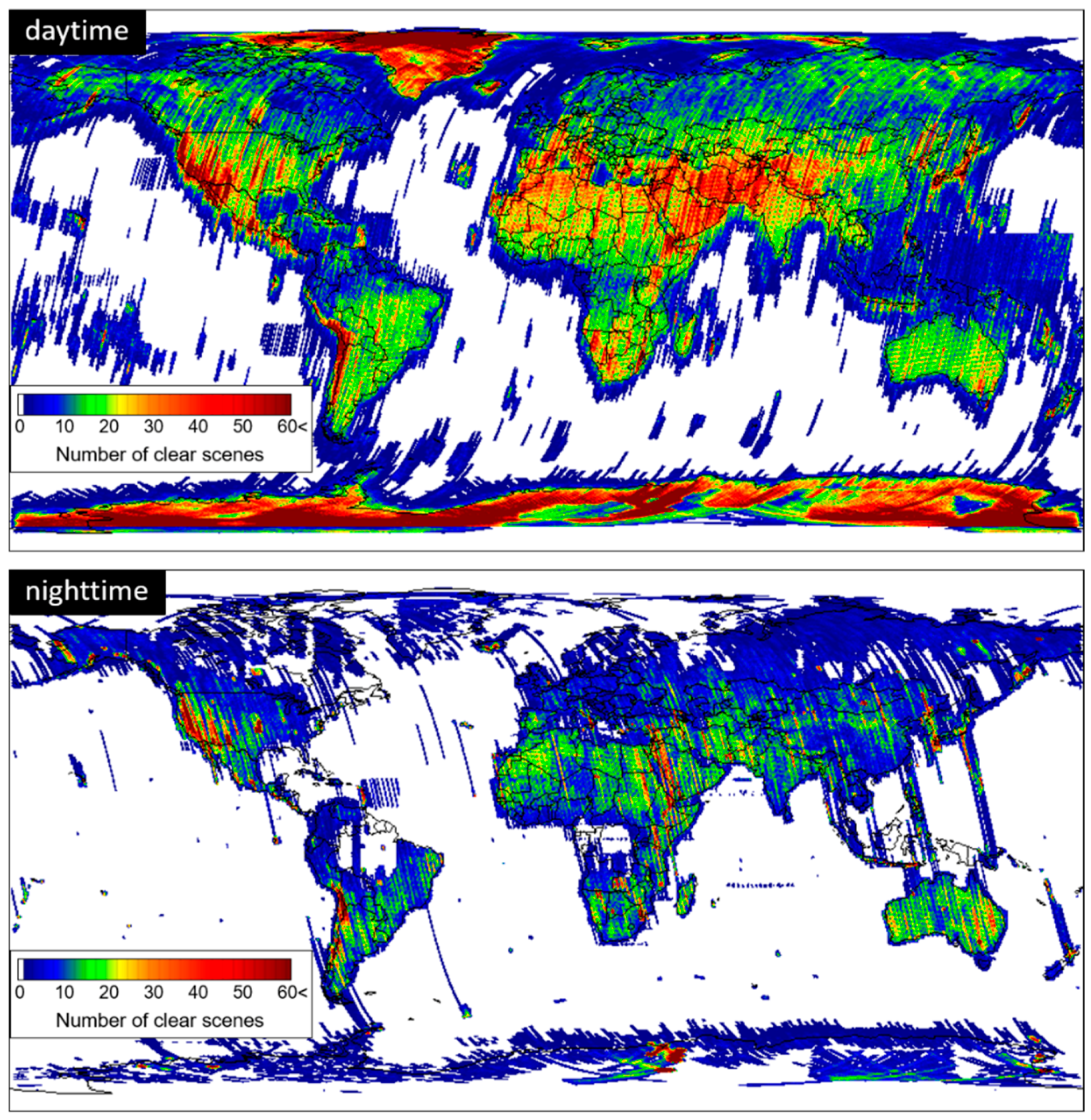
Daytime and nighttime maps of the number of clear scenes with a CC of 20% or less over 10 × 10 degree grids in 19.5 years from March 2000 to August 2019. — Fig. 4.1 Daytime and nighttime maps of the number of clear scenes with a CC of 20% or less over 10 × 10 degree grids in 19.5 years from March 2000 to August 2019 [20].¶

Tip

Accessing ASTER L1A data (Since 2000, 15m resolution, 16 days revisit time) could be possible though the following link: https://www.earthdata.nasa.gov/.

4.4. About the study site - Cordillera Blanca¶

The Cordillera Blanca (Fig. 4.2) is a 200-km-long tropical mountain range in the Peruvian Andes (8°08’-9°58’ S; 77°00’-77°52’ W). The Cordillera Blanca is the most extensive tropical ice-covered mountain range in the world and has the largest concentration of ice in Peru. It hosts several >6,000 m peaks and hundreds of glaciers (area ~723 km²). Most glaciers (530) draining westward covering an area of 507.5 km², while 192 glaciers drains eastern convering 215.9 km² [21]. Like other Andean glaciers, it has experienced pronounced 20th-21st century retreat [22].

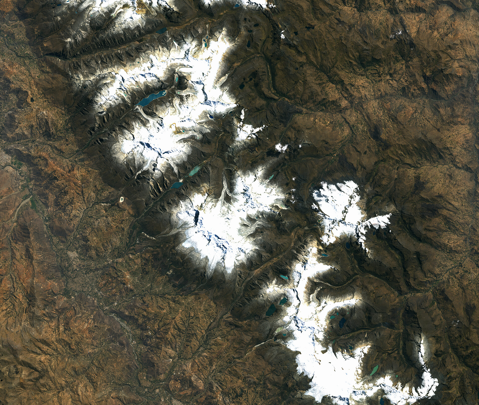
Fig. 4.2 Aerial view of Cordillera Blanca on 24 August 2020. Source: ESA Multimedia¶

Note

In this practice, we will learn how to automatically generate DEM’s by using ASTER images. In order to improve the quality of the results, we will use a SRTM DEM as base to improve uncertainties.

4.5. Download SRTM data¶

First we need to download SRTM tiles (Fig. 4.3). To download SRTM tiles, you need to create an account on the NASA Earthdata web portal. Once you have access to NASA Earthdata, go to the 30-meter SRTM tile downloader and select the tiles you are interested in. Select the tile and click the green download button.

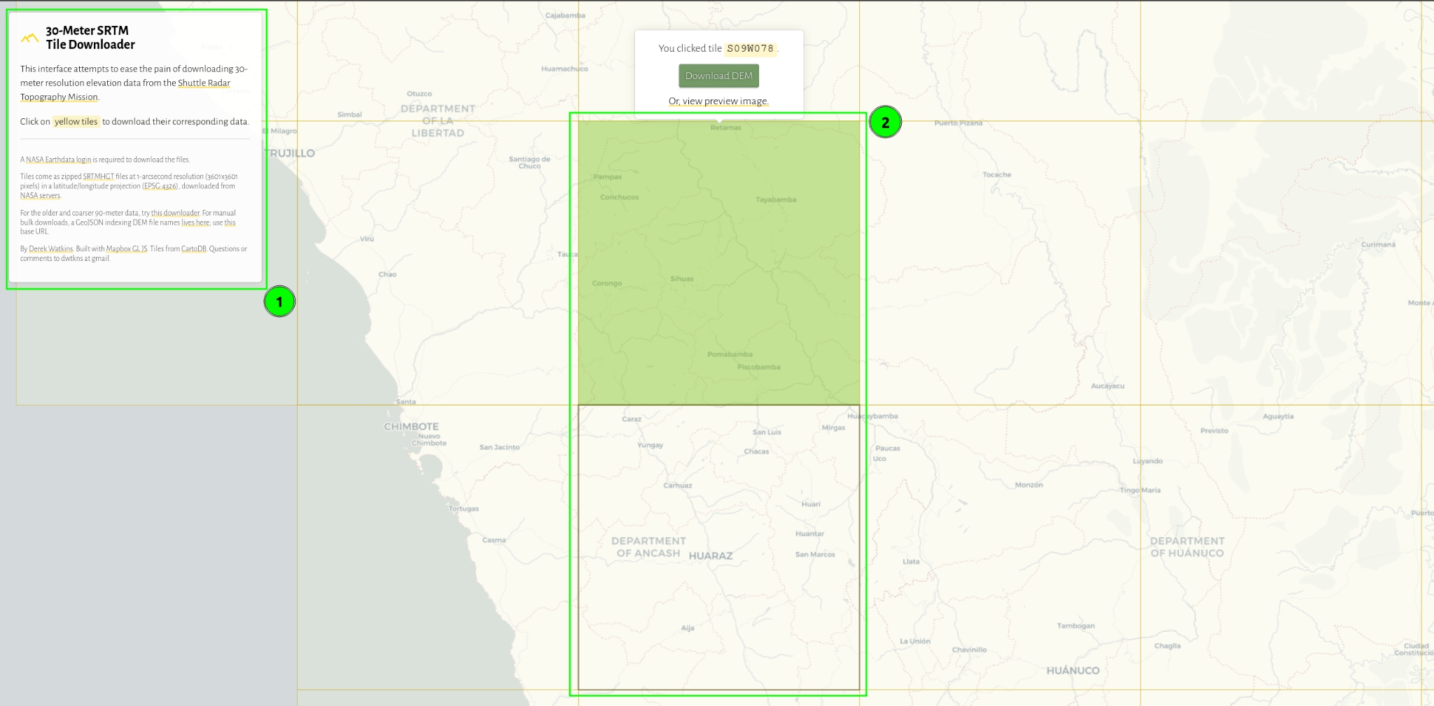
Fig. 4.3 Download SRTM tiles from 30-Meter SRTM Tile Downloader.¶

Important

As the activation of EarthData can take a long time, we already provide SRTM tiles. for this excersice we will use two tiles with codes ‘S09W078’ and ‘S10W078’ Fig. 4.3. You can find the data in the directory DATA/DEM_GENERATION/SRTM_DEM.

4.6. Hands-on¶

4.6.1. Download data for exercise¶

Important

Download the data for this exercise from the following commands:

cd ~/psf_telrisknat_2025_docs/data # Change directory

bash ./download_excercise_3_data.sh # Download data for exercise 3

In order to properly use the SRTM tiles as a seed DEM, we need to take some additional steps to prepare them: Extract the files inside the zip files. To do this, use the following commands:

4.6.2. Prepare SRTM data¶

base_directory="~/psf_telrisknat_2025_docs/data/excercise_3_dems_generation"

cd $base_directory/SRTM_DEM/CBLANCA # Change directory to SRTM_DEM/CBLANCA

for f in *.zip; do unzip "$f"; done # Unzip zip files using for loop

Once the data extracted, you will notice that the tiles use a Hierarchical Data Format (HDF). You can import the files into any GIS software (QGIS for instance). For this exercise, we need to merge all the *.hdf files to have a single GeoTIFF raster file. To do this we will use the Geospatial Data Abstraction Library, commonly known as GDAL. To do this, run the next command:

gdal_merge.py *.hgt -o merged_DEM.tif -of GTiff # Merge all hgt files

By default, the merged DEM has the standard WGS84 georeference. You need to set it up correctly by using a metric georeference (i.e. WGS84 | UTM 18S for the Cordillera Blanca). To do this, run the next command:

gdalwarp -s_srs EPSG:4326 -t_srs EPSG:32718 -r bilinear -of GTiff merged_DEM.tif DEM_REF_for_ASP.tif # Merge all hgt files

You can use the command gdalinfo command to check the results. If you dont feel confortably with comand-line interface, you can import the DEM into QGIS and then look at their properties.

Finally, go back to the base directory.

cd $base_directory

4.6.3. Download ASTER data¶

Now we will know how to download ASTER images. First you need to create an account on the NASA Earthdata portal. Go to the NASA Earthdata data search portal and log in. Using the map background, locate your area of interest and place a marker on the map using the tools on the right. Then search for the collection ASTER L1A Reconstructed Unprocessed Instrument Data V003 and click on it (Figure 4). There are several options available on the toolbar, but a single point-marker is sufficient to select our area of interest (Fig. 4.4).

Once the collection is open and the marker placed, you have access to the tiles that intersect the marker. You are able to filter the data by granule ID (if you know it previously), date range, cloud cover, and so on. You can now select the image of interest. Once you have selected the images, you can add them to the cue and download them all (green button in Fig. 4.4). In the ‘Processing Options’ section, make sure the data format is set to GeoTIFF. Once the download is started, the EarthData web portal will prepare your data and you will receive an email with the download link.

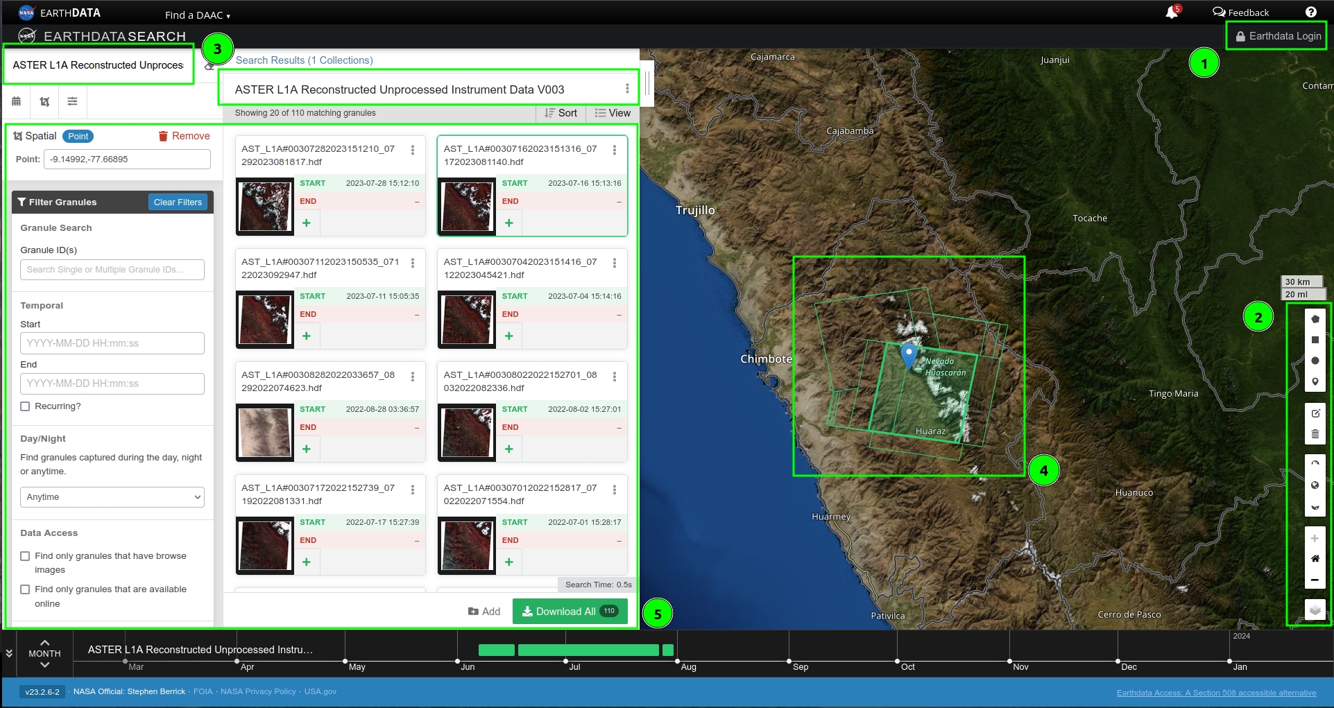
Downloading ASTER images from NASA Earthdata portal. — Fig. 4.4 Download ASTER images from the NASA Earthdata portal.¶

Important

Depending on the amount of granules selected, data preparation can take a long time. For this practice, we already provide several pairs of images over the Cordillera Blanca and Maca region.

4.6.4. Step-by-step automatic DEM generation using ASP¶

For this first part of the exercise, you will work using a recent ASTER image acquired on 4th, July 2023. The ASTER sensor has 15 bands in different spectral ranges. Please refer to the ASTER User Handbook for more detailed and complete information. You can use QGIS software to visualize each one of these bands by clicking on Layer -> Add Raster Layer.

4.6.4.1. Prepare ASTER images¶

We will first use the aster2asp command to prepare the ASTER images. This command takes an input directory of ASTER images and associated metadata, and creates GeoTIFF and XML files that can then be passed to stereo to create a point cloud. The tool can only handle Level 1A ASTER images.

cd $base_directory # Change directory

First, we will copy the ASTER images to a new directory called RAW_L1A. This step is important as the aster2asp command will create several intermediate files in this directory.

mkdir RAW_L1A # Create directory called RAW_L1A

Then, you will decompress the files using the following command:

cd RAW_L1A # Change directory to RAW_L1A

unzip *.zip # Unzip all zip files

Now, you are ready to run the aster2asp command. This command takes as input the directory where the ASTER images are stored (i.e. RAW_L1A) and creates a new directory with the formatted images. You also need to specify the minimum and maximum height of the area of interest using the parameters --min-height and --max-height. For the Cordillera Blanca, we will use 100 m and 9000 m, respectively.

aster2asp RAW_L1A -o RAW_L1A/out_first --min-height 100 --max-height 9000 # Run aster2asp command

As a result of the previous commands, the RAW_L1A directory is created. Within this folder, you will find the formatted stereo pair with the following names: - out-Band3B.tif & out-Band3B.xml, corresponding to the backward image. - out-Band3N.tif & out-Band3N.xml, corresponding to the nadir image.

The process takes a few seconds (~8’’) for the current tile (5000x5400 pixels).

Attention

Pay attention to correctly naming the output files on the parameter -o RAW_L1A/out_first. In this command, you are naming the results as out-first to distinguish from the rest.

Finally, you can clean the RAW_L1A directory by removing the unnecessary files (i.e. *.txt and *.tif files).

rm RAW_L1A/AST_L1A*.txt RAW_L1A/AST_L1A*.tif # Remove unnecessary files

4.6.4.2. Orthorectify images¶

The next step is to orthorectify the formatted images to the seed DEM, e.g. the SRTM DEM we downloaded and prepared in Download SRTM data. To do this, we will use the mapproject command within ASP, as shown below, for both nadir and backward images. The mapproject command takes several arguments such as the rpc session, the georeference option (WGS84 | UTM Zone 18S), the resolution of the map-projected images (i.e. 7.5m), and the seed SRTM DEM.

mapproject -t rpc --t_srs "+proj=utm +zone=18 +south +units=m +datum=WGS84" --mpp 7.5 SRTM_DEM/CBLANCA/DEM_REF_for_ASP.tif RAW_L1A/out_first-Band3N.tif RAW_L1A/out_first-Band3N.xml RAW_L1A/out_first-Band3N_proj_SRTM.tif

mapproject -t rpc --t_srs "+proj=utm +zone=18 +south +units=m +datum=WGS84" --mpp 7.5 SRTM_DEM/CBLANCA/DEM_REF_for_ASP.tif RAW_L1A/out_first-Band3B.tif RAW_L1A/out_first-Band3B.xml RAW_L1A/out_first-Band3B_proj_SRTM.tif

4.6.4.3. Dense stereo matching¶

Run ASP stereo to compute the point cloud (PC). The stereo command takes as input the orthorectified images and their associated XML files. This command produces an point cloud image that can be converted into a visualisable mesh or gridded DEM.

stereo -t astermaprpc --corr-kernel 7 7 --subpixel-kernel 13 13 \
    --alignment-method none \
    RAW_L1A/out_first-Band3N_proj_SRTM.tif \
    RAW_L1A/out_first-Band3B_proj_SRTM.tif \
    RAW_L1A/out_first-Band3N.xml RAW_L1A/out_first-Band3B.xml \
    ASTER_DEM/out_run SRTM_DEM/CBLANCA/DEM_REF_for_ASP.tif

This process creates a directory called ASTER_DEM which contains several intermediate files created by ASP. Please refer to the ASP stereo documentation for more details. The most important file for this exercise is the one ending in *PC.tif, which contains information about the point cloud created during the dense stereo matching process.

4.6.4.4. Convert point cloud to DEM¶

Finally, we will convert the point cloud into a DEM using the point2dem command. This command takes as input the point cloud image and creates a gridded DEM. The output DEM will be in GeoTIFF format.

point2dem -r earth --t_srs "+proj=utm +zone=18 +south +units=m +datum=WGS84" \
    --search-radius-factor 1.5 --tr 30. --nodata-value -9999 \
    ASTER_DEM/out_run-PC.tif -o ASTER_DEM/out_run

An intermediate step with GDAL needs to be executed to correctly setup data type to Float32 bits.

gdal_translate -ot Float32 ASTER_DEM/out_run-DEM.tif ASTER_DEM/first_DEM.tif

4.6.4.5. Setting vertical datum (optional)¶

By default, the DEM generated by ASP is referenced to the WGS84 ellipsoid. However, for most applications, it is preferable to have the DEM referenced to a vertical datum such as EGM96 or EGM2008. To do this, we will use the dem_geoid tool to compute the geoid height at each pixel of the DEM.

dem_geoid ASTER_DEM/first_DEM.tif --geoid EGM96 -o ASTER_DEM/first_DEM_EGM96 # Setting vertical datum to EGM96

gdal_translate -ot Float32 ASTER_DEM/first_DEM_EGM96-adj.tif ASTER_DEM/DEM_20230704.tif # Convert to Float32

Finally, you can clean the ASTER_DEM directory by removing the unnecessary files (i.e. *PC.tif, *DEM.tif, and *DEM-adj.tif files).

rm ASTER_DEM/out_run* ASTER_DEM/first_DEM*

4.6.4.6. Visualize the results¶

Once the results are generated, you should be able to visualize the results using QGIS. You can also use the gdalinfo command to check the properties of the generated DEM. Your results should be similar to the one shown in Fig. 4.5.

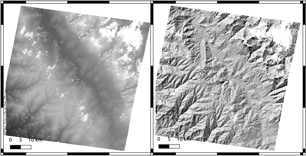
Fig. 4.5 DEM generated from ASTER images using ASP. Left: DEM visualisation; Right: DEM using hillshade effect; visualized in QGIS.¶

Questions for discussion

Based on your experience in this practice, answer the following questions:

What is the noise level of your dataset ?
What do you think about the white holes in the upper right region?
Can you detect differences between ASTER DEM and SRTM DEM?
What do you think is the main limitation of ASTER images?
What are the advantages of using ASP for DEM generation?

4.6.5. Repeat the process with different ASTER images¶

Do it yourself

Repeat the previous steps using another ASTER image acquired on 13th, July 2003 (almost 20 years before). The data are available in the directory RAW_L1A/out_second. Name the output files as out_second to distinguish from the previous results. This step is important as we will use this second DEM to compute the difference of DEMs (DoD) in the next section.

4.6.6. Compute difference of DEMs (DoD)¶

Once the second DEM is processed, you will now compute the Difference of DEMs (DoD). First, as both DEMs have different spatial extents, you need to homogenize into a common spatial extent. To do so, we will use the gdalwarp tool within the GDAL library.

cd ASTER_DEM

common_extent='168757.0 8940932.0 222493.0 9010173.0' # Define common extent

gdalwarp -r bilinear -te $common_extent -of GTiff DEM_20230704.tif DEM_20230704_crop.tif # Cropping first DEM

gdalwarp -r bilinear -te $common_extent -of GTiff DEM_20030713.tif DEM_20030713_crop.tif # Cropping second DEM

Then, you will use the module of raster calculator gdal_calc.py within GDAL to compute the difference of DEMs.

gdal_calc.py -A DEM_20030713_crop.tif -B DEM_20230704_crop.tif --outfile DoD_2023-2003.tif --calc="B-A"

The command gdal_calc.py will generate a new raster file containing the difference between the two generated DEMs. Open this raster in QGIS software. Modify the color scale values Min and Max values of the band between -50 and +50. You should obtain something similar to Fig. 4.6.

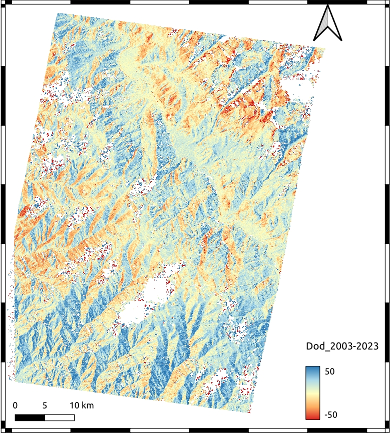
Fig. 4.6 Difference of DEMs (DoD) generated from ASTER images using ASP between 2003 and 2023. Visualized in QGIS.¶

Questions for discussion

Based on your experience in this practice, answer the following questions:

What is the noise level of your dataset ?
What do you think about the white holes in the upper right region?
Can you detect differences between ASTER DEM and SRTM DEM?
What do you think is the main limitation of ASTER images?
What are the advantages of using ASP for DEM generation?

4.7. To go further (bonus)¶

As mentioned in Section 3.4, the processing of ASTER L1A RAW images has become standard in recent years. Together with the DEM_GENERATION dataset, we provide a bash script called make_ASTER-DEM_ASP.sh, which is used to automatically process multiple ASTER images by running a single script. This is based on the [23] and [17] studies and was modified/adapted for this practice. To run this command, first copy all the ASTER tiles you want to process into the same folder (e.g. RAW_L1A). Then go to the parent directory and run the following command indicating the folder where images are stored and the seed DEM:

bash ./make_ASTER-DEM_ASP.sh RAW_L1A SRTM_DEM/CBLANCA/DEM_REF_for_ASP.tif

Do it yourself!!

Congratulations!! Now you have the basic knowledge on how to compute ASTER DEM automatically using ASP. To go further:

Replicate the same process using other ASTER images available in the directory RAW_L1A.
Replicate the same process for another region. You can use the data provided in the directory IMG_MACA.

4.8. References¶

[1]

Joan A. Casey, Yuqian M. Gu, Lara Schwarz, Timothy B. Frankland, Lauren B. Wilner, Heather McBrien, Nina M. Flores, Arnab K. Dey, Gina S. Lee, Chen Chen, Tarik Benmarhnia, and Sara Y. Tartof. The 2025 Los Angeles Wildfires and Outpatient Acute Healthcare Utilization. medRxiv, pages 2025.03.13.25323617, March 2025. doi:10.1101/2025.03.13.25323617.

[2]

Jon E. Keeley and Alexandra D. Syphard. Large California wildfires: 2020 fires in historical context. Fire Ecology, 17(1):22, August 2021. doi:10.1186/s42408-021-00110-7.

[3]

Pascal Lacroix, Gael Araujo, James Hollingsworth, and Edu Taipe. Self-Entrainment Motion of a Slow-Moving Landslide Inferred From Landsat-8 Time Series. Journal of Geophysical Research: Earth Surface, 124(5):1201–1216, 2019. _eprint: https://agupubs.onlinelibrary.wiley.com/doi/pdf/10.1029/2018JF004920. URL: https://onlinelibrary.wiley.com/doi/abs/10.1029/2018JF004920 (visited on 2023-03-01), doi:10.1029/2018JF004920.

[4]

Laura Parra García, Gianluca Furano, Max Ghiglione, Valentina Zancan, Ernesto Imbembo, Christos Ilioudis, Carmine Clemente, and Paolo Trucco. Advancements in Onboard Processing of Synthetic Aperture Radar (SAR) Data: Enhancing Efficiency and Real-Time Capabilities. IEEE Journal of Selected Topics in Applied Earth Observations and Remote Sensing, 17:16625–16645, 2024. doi:10.1109/JSTARS.2024.3406155.

[5]

Diego Cusicanqui, Antoine Rabatel, Christian Vincent, Xavier Bodin, Emmanuel Thibert, and Bernard Francou. Interpretation of Volume and Flux Changes of the Laurichard Rock Glacier Between 1952 and 2019, French Alps. Journal of Geophysical Research: Earth Surface, 126(9):e2021JF006161, October 2021. doi:10.1029/2021JF006161.

[6]

Yifei Zhu, Xin Yao, Leihua Yao, and Chuangchuang Yao. Detection and characterization of active landslides with multisource SAR data and remote sensing in western Guizhou, China. Natural Hazards, 111(1):973–994, March 2022. doi:10.1007/s11069-021-05087-9.

[7]

Pascal Lacroix, Amaury Dehecq, and Edu Taipe. Irrigation-triggered landslides in a Peruvian desert caused by modern intensive farming. Nature Geoscience, 13(1):56–60, January 2020. Number: 1 Publisher: Nature Publishing Group. URL: https://www.nature.com/articles/s41561-019-0500-x (visited on 2023-03-01), doi:10.1038/s41561-019-0500-x.

[8]

David P. Roy, Haiyan Huang, Rasmus Houborg, and Vitor S. Martins. A global analysis of the temporal availability of PlanetScope high spatial resolution multi-spectral imagery. Remote Sensing of Environment, 264:112586, October 2021. doi:10.1016/j.rse.2021.112586.

[9]

Swann Zerathe, Pascal Lacroix, Denis Jongmans, Jersy Marino, Edu Taipe, Marc Wathelet, Walter Pari, Lionel Fidel Smoll, Edmundo Norabuena, Bertrand Guillier, and Lucile Tatard. Morphology, structure and kinematics of a rainfall controlled slow-moving Andean landslide, Peru. Earth Surface Processes and Landforms, 41(11):1477–1493, 2016. doi:10.1002/esp.3913.

[10]

Noélie Bontemps, Pascal Lacroix, and Marie-Pierre Doin. Inversion of deformation fields time-series from optical images, and application to the long term kinematics of slow-moving landslides in Peru. Remote Sensing of Environment, 210:144–158, June 2018. doi:10.1016/j.rse.2018.02.023.

[11]

Francois Ayoub, Sebastien Leprince, Renaud Binet, Kevin W. Lewis, Oded Aharonson, and Jean Philippe Avouac. Influence of camera distortions on satellite image registration and change detection applications: 2008 IEEE International Geoscience and Remote Sensing Symposium - Proceedings. 2008 IEEE International Geoscience and Remote Sensing Symposium - Proceedings, pages II1072–II1075, December 2008. doi:10.1109/IGARSS.2008.4779184.

[12]

Theodore A. Scambos, Melanie J. Dutkiewicz, Jeremy C. Wilson, and Robert A. Bindschadler. Application of image cross-correlation to the measurement of glacier velocity using satellite image data. Remote Sensing of Environment, 42(3):177–186, December 1992. doi:10.1016/0034-4257(92)90101-O.

[13]

Ross A. Beyer, Oleg Alexandrov, and Scott McMichael. The ames stereo pipeline: nasa's open source software for deriving and processing terrain data. Earth and Space Science, 5(9):537–548, 2018. doi:10.1029/2018EA000409.

[14]

David E. Shean, Oleg Alexandrov, Zachary M. Moratto, Benjamin E. Smith, Ian R. Joughin, Claire Porter, and Paul Morin. An automated, open-source pipeline for mass production of digital elevation models (dems) from very-high-resolution commercial stereo satellite imagery. ISPRS Journal of Photogrammetry and Remote Sensing, 116:101–117, 2016. doi:10.1016/j.isprsjprs.2016.03.012.

[15]

Diego Cusicanqui, Pascal Lacroix, Xavier Bodin, Benjamin Aubrey Robson, Andreas Kääb, and Shelley MacDonell. Detection and reconstruction of rock glacier kinematics over 24 years (2000–2024) from Landsat imagery. The Cryosphere, 19(7):2559–2581, July 2025. doi:10.5194/tc-19-2559-2025.

[16]

Martin Mergili, Adam Emmer, Anna Juřicová, Alejo Cochachin, Jan-Thomas Fischer, Christian Huggel, and Shiva P. Pudasaini. How well can we simulate complex hydro-geomorphic process chains? The 2012 multi-lake outburst flood in the Santa Cruz Valley (Cordillera Blanca, Perú). Earth Surface Processes and Landforms, 43(7):1373–1389, 2018. doi:10.1002/esp.4318.

[17] (1,2)

I. Dussaillant, E. Berthier, F. Brun, M. Masiokas, R. Hugonnet, V. Favier, A. Rabatel, P. Pitte, and L. Ruiz. Two decades of glacier mass loss along the andes. Nature Geoscience, 12(10):802–808, 2019. doi:10.1038/s41561-019-0432-5.

[18]

D. Schneider, C. Huggel, A. Cochachin, S. Guillén, and J. García. Mapping hazards from glacier lake outburst floods based on modelling of process cascades at lake 513, carhuaz, peru. In Advances in Geosciences, volume 35, 145–155. 2014. URL: https://adgeo.copernicus.org/articles/35/145/2014/, doi:10.5194/adgeo-35-145-2014.

[19]

Diego Cusicanqui and Xavier Bodin. Photogrammetry for the study of mountain slopes. Webinar at INDURA, 2019. URL: https://vimeo.com/473376992.

[20]

Hideyuki Tonooka and Tetsushi Tachikawa. Aster cloud coverage assessment and mission operations analysis using terra/modis cloud mask products. Remote Sensing, 11(23):2798, 2019. doi:10.3390/rs11232798.

[21]

INAIGEM. Inventario nacional de glaciares y lagunas de origen glaciar 2023. Technical Report, Instituto Nacional de Investigación en Glaciares y Ecosistemas de Montaña, 2023. URL: https://hdl.handle.net/20.500.12748/499.

[22]

Romain Hugonnet, Robert McNabb, Etienne Berthier, Brian Menounos, Christopher Nuth, Luc Girod, Daniel Farinotti, Matthias Huss, Ines Dussaillant, Fanny Brun, and Andreas Kääb. Accelerated global glacier mass loss in the early twenty-first century. Nature, 592(7856):726–731, 2021. doi:10.1038/s41586-021-03436-z.

[23]

Fanny Brun, Etienne Berthier, Patrick Wagnon, Andreas Kääb, and Désirée Treichler. A spatially resolved estimate of high mountain asia glacier mass balances from 2000 to 2016. Nature Geoscience, 10(9):668–673, 2017. doi:10.1038/ngeo2999.

[24]

C. Nuth and A. Kääb. Co-registration and bias corrections of satellite elevation data sets for quantifying glacier thickness change. The Cryosphere, 5(1):271–290, March 2011. doi:10.5194/tc-5-271-2011.

[25]

A. Federico, M. Popescu, G. Elia, C. Fidelibus, G. Internò, and A. Murianni. Prediction of time to slope failure: a general framework. Environmental Earth Sciences, 66(1):245–256, May 2012. doi:10.1007/s12665-011-1231-5.

[26]

Mathilde Desrues, Pascal Lacroix, and Ombeline Brenguier. Satellite Pre-Failure Detection and In Situ Monitoring of the Landslide of the Tunnel du Chambon, French Alps. Geosciences, 9(7):313, July 2019. doi:10.3390/geosciences9070313.

[27]

Teruki Fukuzono. A new method for predicting the failure time of slope. In Proceedings, 4th Int'l. Conference and Field Workshop on Landslides, 145–150. 1985.

[28]

M Saito. Forecasting time of slope failure by tertiary creep. In Proceedings of 7th International Conference on Soil Mechanics and Foundation Engineering, 1969, volume 2, 677–683. 1969.

[29]

A. Segalini, A. Valletta, and A. Carri. Landslide time-of-failure forecast and alert threshold assessment: A generalized criterion. Engineering Geology, 245:72–80, November 2018. doi:10.1016/j.enggeo.2018.08.003.